| [Top] | [Contents] | [Index] | [ ? ] |
This document describes the TENNS Neural Simulation Framework (tenns). It is designed for heterogenous models that fit a network paradigm of nodes and connections. It supports the integration of components that conform to the Network Model Interface. This edition documents version 1.53.
1. Notices 2. Introduction 3. Installation 4. Overview 5. Heterogenous Systems 6. About Models 7. Using TENNS 8. Tutorial 9. Troubleshooting Concept Index
-- The Detailed Node Listing ---
Introduction
2.1 Philosophy of Approach 2.2 A Note on User Interfaces 2.3 Companion Software 2.4 Obtaining 2.5 Other Documentation
Installation
3.1 Dependencies 3.2 Platforms 3.3 Required Build Tools 3.4 Building 3.5 Environment
Overview
4.1 Related Packages
Heterogenous Systems
5.1 Current Scope 5.2 Complexity 5.3 Name Spaces 5.4 Integration
About Models
6.1 Objects 6.2 Control 6.3 Naming
Naming
6.3.1 Expansion of Names 6.3.2 Set Constructs
Using TENNS
Understanding the Frontend
7.1.1 Configuration Scripts 7.1.2 Frontend Usage 7.1.3 The Frontend Pre-processor 7.1.4 Binding to a Backend 7.1.5 The .rc File 7.1.6 Structure of the Frontend 7.1.7 Libraries
Scripting Language Commands
7.3.1 Object Related Commands 7.3.2 House-keeping Commands
Getting Help Online
7.6.1 Help on Scripting Language 7.6.2 Class Definitions 7.6.3 Help on Global Commands
Tutorial
8.1 Getting Started 8.2 A Cerebellar Smooth Eye Pursuit Example 8.3 A Cerebellar Granular Layer Learning Example
| [ < ] | [ > ] | [ << ] | [ Up ] | [ >> ] | [Top] | [Contents] | [Index] | [ ? ] |
The TENNS Neural Simulation Framework
Copyright (C) 1997 - 2003 Mike Arnold, Altjira Software, 2002 - 2003 Mike Arnold, The Salk Institute for Biological Studies
Permission is granted to make and distribute verbatim copies of this manual provided the copyright notice and this permission notice are preserved on all copies.
This software and documentation is provided "as is" without express or implied warranty. All questions should be addressed to mikea@altjira.com.
| [ < ] | [ > ] | [ << ] | [ Up ] | [ >> ] | [Top] | [Contents] | [Index] | [ ? ] |
The TENNS Neural Simulation Framework is designed for heterogenous models that fit a network paradigm of nodes and connections. It supports the integration of components that conform to the Network Model Interface.
2.1 Philosophy of Approach 2.2 A Note on User Interfaces 2.3 Companion Software 2.4 Obtaining 2.5 Other Documentation
| [ < ] | [ > ] | [ << ] | [ Up ] | [ >> ] | [Top] | [Contents] | [Index] | [ ? ] |
Traditionally discussions of the constraints on the computer simulation of neural structures have been dominated by the computation and communication costs. Such discussions have been based on the requirement to model compact homogenous structures with possibly a single learning algorithm. The coherent nature of the brain implies that the usefulness of a functional analysis of a brain area in isolation can be limited. Furthermore, the brain can be usefully modelled at different levels of abstraction, using different structures and algorithms and with differing costs. Simulations in the future could be characterised as 1) being heterogenous and involving different levels of abstraction; 2) requiring a mixture of different learning algorithms with varying scopes; 3) being very large with large numbers of free parameters and 4) depending on the integration of components from different researchers. Mixtures of synchronous and asynchronous data flows, algorithms, and time resolutions increase the complexity of the timing, control and scope issues. Dynamically varying the abstraction or time resolution, locally or globally, complicates the resource allocation problem. Configuration and management of the experimental process becomes a critical constraint. The complexity required of both the software and the user grows more than linearly with the model diversity.
TENNS is a neural simulation framework designed to be scalable with both the size and the complexity of the models. It specifically addresses the complexities that arise from modelling heterogenous networks using multiple paradigms, synchronous and asynchronous data flows, multiple learning algorithms with varying data scopes, different approaches to parallelisation, and the integration with models and systems running in either 3rd party software or dedicated hardware.
TENNS is an object-oriented parallel-computing application. It runs under shared memory architectures, using the POSIX pthreads library, and under distributed memory architectures, using MPI.
| [ < ] | [ > ] | [ << ] | [ Up ] | [ >> ] | [Top] | [Contents] | [Index] | [ ? ] |
TENNS does not have a graphical user interface. It uses instead a commandline interface. It does not have a graphical frontend. A single instance of TENNS may have multiple commandline sessions running concurrently. An optional script-based frontend written as a set of GNU Bash shell scripts is also supplied. TENNS does not have any builtin visualisation tools for viewing results, but instead writes all data to text files which can be imported into programs such as matlab or openDX for post-processing. The post-processing of data generated by TENNS can be facilitated using the Data Extraction Library.
| [ < ] | [ > ] | [ << ] | [ Up ] | [ >> ] | [Top] | [Contents] | [Index] | [ ? ] |
TENNS is based on the Network Model Interface library. As such it supports the integration of components based on the library. For a list of available components and their associated support file packages, and information regarding interoperability, refer to the libnmi documentation and the NMI Simulation Resources documentation.
Separate software that works with TENNS includes the Data Extraction Library (libdext) for post-processing TENNS generated data files. The post-processed data can be imported in to Matlab for further proccessing and visualisation using the matdpp Matlab Wrapper routines for libdext.
The following support file packages are also available for TENNS (also check the NMI Simulation Resources documentation). Note that TENNS related files will also be available within the support file packages associated with any libnmi-derived components.
| [ < ] | [ > ] | [ << ] | [ Up ] | [ >> ] | [Top] | [Contents] | [Index] | [ ? ] |
TENNS may be downloaded from http://www.altjira.com/distrib/tenns. See also 3.1 Dependencies, and 2.3 Companion Software, for other software that may need to be downloaded and installed.
The latest version of this documentation may be found at http://www.altjira.com/support/tenns/tenns.html.
| [ < ] | [ > ] | [ << ] | [ Up ] | [ >> ] | [Top] | [Contents] | [Index] | [ ? ] |
A reference manual. describing the classes within TENNS is available in html format. The latest version of this reference manual may be found at http://www.cnl.salk.edu/~mikea/doc/tenns/reference/tennsS-ref-toc.html.
Information is also available within TENNS (7.6 Getting Help Online), detailing the command syntax and the available object classes.
Examples and tutorials can be found within the support file packages listed in 2.3 Companion Software.
This documentation is also installed to ${prefix}/doc/tenns, where `${prefix}' is the installation directory specified during the build configuration.
| [ < ] | [ > ] | [ << ] | [ Up ] | [ >> ] | [Top] | [Contents] | [Index] | [ ? ] |
3.1 Dependencies 3.2 Platforms 3.3 Required Build Tools 3.4 Building 3.5 Environment
| [ < ] | [ > ] | [ << ] | [ Up ] | [ >> ] | [Top] | [Contents] | [Index] | [ ? ] |
TENNS is built on the ANSI Standard C++ Library and the POSIX pthreads library. It also requires the following libraries to be already installed.
Other libraries may be required depending on the optional packages to be enabled see section 2.3 Companion Software. See the README file in the distribution for the definitive list of available packages.
The optional script based frontend requires GNU m4 version 1.4 or later and the bash command shell.
| [ < ] | [ > ] | [ << ] | [ Up ] | [ >> ] | [Top] | [Contents] | [Index] | [ ? ] |
TENNS has been successfully tested on the following systems:
| [ < ] | [ > ] | [ << ] | [ Up ] | [ >> ] | [Top] | [Contents] | [Index] | [ ? ] |
The following software is suggested. Other versions may work but have not been tested.
Package maintenance requires:
| [ < ] | [ > ] | [ << ] | [ Up ] | [ >> ] | [Top] | [Contents] | [Index] | [ ? ] |
Refer to the README and INSTALL files in the distribution.
| [ < ] | [ > ] | [ << ] | [ Up ] | [ >> ] | [Top] | [Contents] | [Index] | [ ? ] |
The TENNS environment can be configured using the following files, where `${prefix}' is the installation directory specified during the build configuration:
Neither of these files need be sourced by the user's login script.
Instead they are sourced as required when TENNS runs.
TENNS does not require any variables to be exported from the user's environment.
The use of environment variables such as TENNSHOME that had to be set prior to running TENNS has been deprecated since version 1.51.
Both files are used primarily to define the M4PATH environment variable.
M4PATH is used by TENNS to determine where it should look for project files (for details refer to 7.1.3 The Frontend Pre-processor).
M4PATH should include the path to all the library files installed with any support file packages (see 2.3 Companion Software).
An alternative user-specific configuration file may be specified as a commandline option when starting the frontend (for details refer to 7.1.5 The .rc File).
Here is a typical `.tennsrc' file:
# user specific TENNS configuration file
# do not source this file at login

source ${TENNSDATA}/tenns.rc
M4PATH=${M4PATH}:/usr/local/share/nmisim/tenns/runpkg
M4PATH=${M4PATH}:${HOME}/projects/my-project
|
Note that the following line must be included:
source ${TENNSDATA}/tenns.rc
|
The environment variable TENNSDATA is set by TENNS and does not need to be set by the user prior to running TENNS.
Similarly, there is no need for the user to export M4PATH, as it will be exported by TENNS as required.
To use the matlab engine in libmtng one may need to set the environment variable LD_LIBRARY_PATH in the user's shell, for example:
LD_LIBRARY_PATH=${LD_LIBRARY_PATH}:/usr/local/matlab/extern/lib/glnx86:/usr/local/matlab/sys/os/glnx86
|
Check the matlab documentation.
| [ < ] | [ > ] | [ << ] | [ Up ] | [ >> ] | [Top] | [Contents] | [Index] | [ ? ] |
4.1 Related Packages
| [ < ] | [ > ] | [ << ] | [ Up ] | [ >> ] | [Top] | [Contents] | [Index] | [ ? ] |
Support file packages for TENNS and for any libnmi-derived components should be installed as indicated in the NMI Simulation Resources documentation.
After installing a package the M4PATH environment variable should be modified in the `${HOME}/.tennsrc' user specific configuration file, to include the path for the library files in the new package.
| [ < ] | [ > ] | [ << ] | [ Up ] | [ >> ] | [Top] | [Contents] | [Index] | [ ? ] |
The aim of the simulator is to manage the complexity the simulation process as the complexity of the model increases. The complexity of the model may increase with the size of the model, the complexity of the network architecture, the number, diversity and scope of the learning algorithms, the number of different neural paradigms, the number and diversity of different hardware computer platforms and hardware implementations, and the number and diversity of physical and functional systems that can be coupled to the model.
Importantly the aim of the simulator is to manage the complexity as these diverse resources and elements are combined together within single hybrid simulations. This corresponds to the traditional simulation environments that are designed for homogenous models consisting of a single neural paradigm, a single temporal paradigm, a single or no learning algorithm and simple network architectures.
5.1 Current Scope 5.2 Complexity 5.3 Name Spaces 5.4 Integration
| [ < ] | [ > ] | [ << ] | [ Up ] | [ >> ] | [Top] | [Contents] | [Index] | [ ? ] |
Currently this complexity covers:
| [ < ] | [ > ] | [ << ] | [ Up ] | [ >> ] | [Top] | [Contents] | [Index] | [ ? ] |
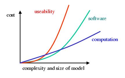
The cost as the complexity of the model increases can be measured at 3 different points; as the computational cost, as the software cost, and as the useability cost.
The computational cost is addressed by using a mixture of distributed memory and shared memory mechanisms, specifically by using MPI and Posix threads. The model is segmented up into components to reflect the requirements for the communication of data between objects and the sharing of objects in memory. Inter-component communication is implemented through channel objects which can be derived for inter-process or inter-thread communication. Computation for objects within a component context is on a shared memory model. Load balancing is implemented through the transfer between components.
The software cost is addressed through the use of an object-oriented language, C++. The use of templates reduces the need for virtual functions.
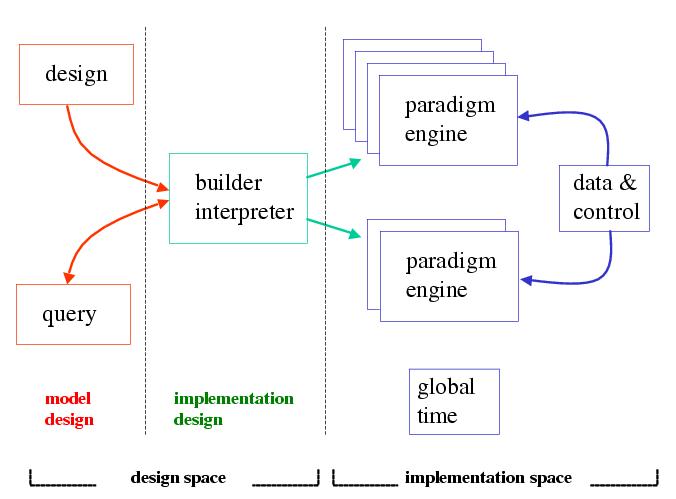
The useability cost is considered to be the least scaleable. Useability is dependent on the the reuseability of the configuration code as the model space is explored. The key element in dealing with the useability cost is to divide the objects in a model into a design space and an implementation space. Objects in the design space define the model within the language of the experimenter. The design space also includes build objects that define the how the design is to be implementated or built. The implementation consists of a single controller object and a set of components. Each component is the root of a tree of objects which collectively implement the functionality required of that component. The grouping of implementation related objects in to trees reflects the grouping of the objects under the specified memory model. Objects within a tree are considered to share the same address space. All communication between trees is explicit through the use of channel objects.
| [ < ] | [ > ] | [ << ] | [ Up ] | [ >> ] | [Top] | [Contents] | [Index] | [ ? ] |
The build objects are used to build the implementation from the design and to communicate between the design objects and the implementation objects. The build objects act as interpreters or translaters between the two spaces. The build objects provide naming mechanisms that allow an object in one space to be referenced with respect to an object in the other space. This is a key element in reducing the useability cost.
For example the synaptic weight of the first synapse in the first node in a network, relative to the network, is referenced by:
node/0/iconn/0/weight |
It is generally more convenient to reference a synaptic weight by its logical name in the design space. For example, the synaptic weight of the synapse to the first node in the Purkinje layer from the first node in the Basket cell layer is given by:
purkinje/node/0/iconn/basket:0/weight |
This allows the implemented objects, corresponding to elements in the design of the model, to be referenced using a single mechanism independently of the implementation.
| [ < ] | [ > ] | [ << ] | [ Up ] | [ >> ] | [Top] | [Contents] | [Index] | [ ? ] |
The simulator includes MPI based constructs that can be wrapped around 3rd party software to facilitate their integration into the TENNS environment.
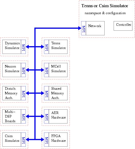
Each resource is integrated at low cost using the MPI wrapper. Resources are ordered in a master-slave relationship, implying that one of the resources must accept the role of master at additional cost. The master is given organisational, coordination, allocation and namespace related functionality. Using MPI allows diverse resources running as distinct processes on heterogenous hardware to be integrated at low cost. The red dotted lines denote process boundaries. The blue lines denote MPI-implemented data buses.
| [ < ] | [ > ] | [ << ] | [ Up ] | [ >> ] | [Top] | [Contents] | [Index] | [ ? ] |
A model is a set of objects. An object is an instantiation of a class. The operation of the simulator involves the creation, configuration and execution of objects of different types.
6.1 Objects 6.2 Control 6.3 Naming
| [ < ] | [ > ] | [ << ] | [ Up ] | [ >> ] | [Top] | [Contents] | [Index] | [ ? ] |
All objects are derived from a common base class, the Particle class. The class hierarchy is arranged as a tree with Particle as the root. Other important base classes are:
| [ < ] | [ > ] | [ << ] | [ Up ] | [ >> ] | [Top] | [Contents] | [Index] | [ ? ] |
The aim of the simulator is to distribute the control of the simulation and to avoid the accumulation of control mechanisms at a single point. The motivation is to avoid the supra-linear increase in complexity that occurs with an omnipotent controller as it is required to coordinate an increasing number of learning algorithms and neural paradigms with different time scales and different scopes. The distribution of the control and scheduling of functions is a key element in ensuring that the simulator can scale in the complexity of the model.
The goal is to manage at a local level, the control of a specific functionality. Data, including temporal information, as well as control can be passed between objects.
An omnipotent control object does exist in order to maintain a global time and ensure the temporal synchronisation between objects. On initialisation the simulation contains only a single object, the default control object with the name "default-controller". The type of this controller can be defined using a commandline option to the backend. Each object of a Component-derived class is bound to a control object, "default-controller" is used by default.
| [ < ] | [ > ] | [ << ] | [ Up ] | [ >> ] | [Top] | [Contents] | [Index] | [ ? ] |
Every object can be referenced using a naming strategy. Some objects have only relative names and can be referenced only with respect to another object. Other objects have absolute names that exist within a global namespace. Currently the global namespace is a flat structure. An object may have only a single absolute name, but it may have multiple relative names.
Each class of objects may have defined a number of different naming mechanisms that can be used to reference relative objects. These are listed in the class description. A naming mechanism is of the form:
<type>/<idenitifier> |
For example "node/0" can be used to reference, relative to a network, the first node in the network.
A relative name is made up of a sequence of naming mechanisms separated by the '/' separator. For example the synaptic weight of the first synapse in the first node in a network, relative to the network, is referenced by:
node/0/iconn/0/weight |
6.3.1 Expansion of Names 6.3.2 Set Constructs
| [ < ] | [ > ] | [ << ] | [ Up ] | [ >> ] | [Top] | [Contents] | [Index] | [ ? ] |
Using object name expansion a naming string is expanded to a set of objects. A number of expansions are tried in the following order, stopping on the first successful expansion:
Data expansion exists as well as name expansion. If <value> is of the form @<object>@ then it is expanded to:
<object>->operator()() |
This is useful for assigning a sample from a distribution to a parameter.
| [ < ] | [ > ] | [ << ] | [ Up ] | [ >> ] | [Top] | [Contents] | [Index] | [ ? ] |
Set or collection constructs are implemented in two ways, through an object of type Set and through object expansion. Sets of objects can be defined and referred to by {<name>} where <name> is the name of a set object.
The set object consists of a definition which is resolved to a set of objects using object expansion. The resolution of the definition can be performed either whenever the set is referenced or at explicit times such as when the definition of the set is modified.
For example a definition may include "Component", which is resolved to all objects of type "Component" at the time of the resolution. Alternatively, definition may include all of the objects of type "Component" at the time of definition, which is always resolved to that same group of objects even if new "Component" objects are later created.
Normal object expansion is used when modifying the definition of a set. This can be avoided by quoting the expansion string. Thus add=Component adds each object of type "Component" that currently exists to the definition, which will always be resolved to the same set of objects even if new Component objects are later created. However add='Component' adds the type "Component" to the definition, which is resolved to all objects of type "Component" at the time of the resolution.
| [ < ] | [ > ] | [ << ] | [ Up ] | [ >> ] | [Top] | [Contents] | [Index] | [ ? ] |
TENNS is comprised of two parts, a backend simulator (tennsS) and a frontend shell (tenns). These may be run in a number of different ways. The backend simulator may be run by itself, or it may be run through the frontend. Alternatively a frontend may be run by itself, and then be made to connect to an already running backend. A frontend may only be connected to a single backend at any one time. A backend though may have multiple frontends connected to it at any one time (for details refer to 7.1.4 Binding to a Backend).
In any of the scenarios, whether communicating through a frontend or communicating directly to a backend, the user sees a very similar commandline interface. The main difference is that the commandline interface for the backend is fairly primitive and fixed, whilst the frontend has a more sophisticated and extendable commandline interface. Generally TENNS will be used through the frontend, except perhaps when debugging or running pre-compiled configuration files in batch mode (see 7.1.1 Configuration Scripts).
To start up the frontend, together with an attached backend, type:
tenns |
or
tenns <sources> - |
where <sources> are a list of configuration files.
In most cases this is sufficient to run a simulation.
A frontend will be started, along with a backend.
The frontend will parse the sources and generate a list of commands which are passed to the backend.
After the sources are parsed, the - tells the frontend to start an interactive session, enabling the user to pass commands through the frontend to the backend (see 7.3 Scripting Language Commands).
| [ < ] | [ > ] | [ << ] | [ Up ] | [ >> ] | [Top] | [Contents] | [Index] | [ ? ] |
The backend works by parsing streams of configuration text according to a simple language. These streams determine the construction of the model and the running of the simulation.
The configuration language for the backend is very simple, with no control flow or variable constructs. The advantage of this is its ease of implementation and that it provides an exact and readable definition of the simulation. The disadvantage of such a simple language is that for complex simulations it is not particularly useable from the modeler's point of view. The configuration files can be very large and tedious to write. For these reasons we have added a frontend built on top of the GNU bash shell. The frontend is not graphical and appears to the user as a commandline interface that looks very similar to the commandline interface of the backend. It is however a commandline interface that has all the power of a bash shell, including the control, variable and function constructs available in bash.
The backend is capable of reading configuration streams from either files, an interactive session, or from a set of binary executables located in ${prefix}/tenns/libexec, where `${prefix}' is the installation directory specified during the build configuration. The frontend communicates through these binary executables. There is an executable for each of the commands in the backend's simple scripting language (see 7.3 Scripting Language Commands).
This mechanism means that the frontend and backend are distinct programs. Indeed, the frontend is simply a set of shell scripts based on the bash shell. The advantages of this approach of using a standard shell as the frontend for the simulator are:
7.1.1 Configuration Scripts 7.1.2 Frontend Usage 7.1.3 The Frontend Pre-processor 7.1.4 Binding to a Backend 7.1.5 The .rc File 7.1.6 Structure of the Frontend 7.1.7 Libraries
| [ < ] | [ > ] | [ << ] | [ Up ] | [ >> ] | [Top] | [Contents] | [Index] | [ ? ] |
The frontend configuration scripts are shell scripts and any valid shell script is a valid frontend configuration script. As both the frontend and the backend use the same comment delimiters, generally any valid backend script is also a valid frontend script. The reverse is not always true, as a frontend script may include constructs that can not be understood directly by the backend.
The frontend works by parsing the configuration scripts as if they were shell scripts, generating a stream of backend specific statements and general system commands. The backend specific statements are passed through to the backend as they are generated.
The backend keeps a record of all the statements it receives via all of its configuration streams in the file `input.dbg'. This file is an exact record of what has happened during the simulation, and can be used to reconstruct the simulation. Note that the file only contains the statements used to generate the simulation, it does not necessarily capture the data that is sampled by the simulation.
The `input.dbg' file may be used to compile a set of frontend configuration scripts by invoking the frontend as a compiler.
In this mode, the frontend parses the configuration scripts as usual, passing them to the backend, and in the process generating the `input.dbg' file.
The frontend invokes the backend with the --compile flag (see 7.2 Running the Backend Directly).
This tells the backend to do run the simulation, doing everything except for the computation when iterating the system forward through time.
This allows a set of configuration scripts to be parsed and verified in a minimal amount of time.
It also generates a backend readable record of the simulation in `input.dbg'.
This compiled record can be useful for running on systems where there is no frontend.
| [ < ] | [ > ] | [ << ] | [ Up ] | [ >> ] | [Top] | [Contents] | [Index] | [ ? ] |
The TENNS simulator is generally run with a frontend using:
tenns [options] [<file> ...] tenns -h |
where <file> is a script or configuration file. If file is equal to '-' then commands will be read from standard input. If no files are supplied then the standard input is used. The following options are supported:
| [ < ] | [ > ] | [ << ] | [ Up ] | [ >> ] | [Top] | [Contents] | [Index] | [ ? ] |
All input to the frontend is first passed through an optional pre-processor, by default the Gnu macro processor m4. The pre-processor can be turned off but is on by default using a commandline option. It maintains a current state of definitions, which is initialised from the definition file ${prefix}/share/tenns/tenns.m4, where `${prefix}' is the installation directory specified during the build configuration.
It is used primarily to provide support for the inclusion of script files within a script, using the m4 include() construct.
The environment variable M4PATH is used to define the search path for included files.
For details on setting M4PATH refer to 3.5 Environment and 7.1.5 The .rc File.
| [ < ] | [ > ] | [ << ] | [ Up ] | [ >> ] | [Top] | [Contents] | [Index] | [ ? ] |
A frontend may bind itself to any backend (for details refer to 7.1.2 Frontend Usage). If no backend is specified as a commandline option, then the frontend will start up a backend and then bind to it.
choose() will list the available backends that can be bound to, and bind the frontend to the chosen backend.
A backend may be bound to multiple frontends. Each frontend has its own command interpreter and associated input/output/error streams within the backend. This allows a backend to be configured and queried through multiple attachable and detachable user interfaces.
| [ < ] | [ > ] | [ << ] | [ Up ] | [ >> ] | [Top] | [Contents] | [Index] | [ ? ] |
The -r option is used to specify the initialisation file that is sourced by the frontend in both interactive and non-interactive modes. The default file, if it exists, is the user-specific configuration file `.tennsrc' file located in the user's home directory. If it does not exist, then the frontend uses the system `tenns.rc' file located in `${prefix}/share/tenns', where `${prefix}' is the installation directory specified during the build configuration. Whatever initialisation file is used, it should always source this system `tenns.rc' file. For details on writing initialisation files refer to 3.5 Environment.
| [ < ] | [ > ] | [ << ] | [ Up ] | [ >> ] | [Top] | [Contents] | [Index] | [ ? ] |
The tenns frontend does the following:
| [ < ] | [ > ] | [ << ] | [ Up ] | [ >> ] | [Top] | [Contents] | [Index] | [ ? ] |
The frontend has a number of library files which package basic functionality. They are located in `${prefix}/share/tenns', where `${prefix}' is the installation directory specified during the build configuration.
| [ < ] | [ > ] | [ << ] | [ Up ] | [ >> ] | [Top] | [Contents] | [Index] | [ ? ] |
The backend tennsS can be run on its own using:
tennsS [options] <file> [<file> ...] tennsS --help tennsS --version |
where <file> is a script file. If file is equal to '-' then commands will be read from standard input. The commandline interface to the backend does not support history or line-editing mechanisms. The following options are supported:
--controller <controller_type> |
Define the class type of the default controller that is used to control the simulation.
--checkpoint |
That the simulation is to initialise itself from the checkpoint file in the current directory.
--cpulimit <t sec> |
Define the amount of cpu time the simulation is to run before writing a checkpoint and exiting.
--chkptcom <string> |
Define the shell command to be executed after writing out the checkpoint and before exiting.
--compile |
That the simulation is to run in compile mode where all computation associated with each time-step is skipped.
| [ < ] | [ > ] | [ << ] | [ Up ] | [ >> ] | [Top] | [Contents] | [Index] | [ ? ] |
TENNS has very few commands that can be given at the commandline, primarily only commands to create, delete, list, configure and execute objects, as well as various house-keeping commands. Note that each class does have its own set of commands, however these are accessed through the execute object command (for details refer to 7.4 Using Classes and 7.6.2 Class Definitions). There are also a set of object related commands, termed global commands, that are also accessed through the execute object command (for details refer to 7.5 Global Commands and 7.6.3 Help on Global Commands).
The syntax of the TENNS scripting language is the same whether it is entered through a frontend or directly to the backend. Commands end with a newline. Only in the frontend can commands also end with a semicolon. Commands in the frontend separated by a semicolon are sent to the backend on separate lines.
7.3.1 Object Related Commands 7.3.2 House-keeping Commands
| [ < ] | [ > ] | [ << ] | [ Up ] | [ >> ] | [Top] | [Contents] | [Index] | [ ? ] |
The following commands manage objects:
ex <identifier> <command> [input>:<output>] <arguments ...]
execute the specified <command> for each of the objects referenced by <identifier>
ex global <command> [stream <input>:<output>] <arguments ...]
execute the specified global <command>
ex <identifier>
execute the default operator (the default command) for each of the objects referenced by <identifier>.
config <identifier> <config-string> ... [+]
configure each of the objects referenced by <identifier> with the specified <config-string>. If the optional + suffix is supplied, then also call the default operator for each of the objects after applying the configuration. Multiple <config-string> may be specified.
create <type> <name> [config-string] [+]
create an object of the specified <type> within the current namespace and with the specified <name>. The object may then be configured with the optional <config-string>. If the + suffix is specified, then the default operator for the object is called after any configuration.
list [<identifier> ...]
list the objects referenced by <identifier>. If <identifier> is not given then list all the objects in the namespace.
| [ < ] | [ > ] | [ << ] | [ Up ] | [ >> ] | [Top] | [Contents] | [Index] | [ ? ] |
The following commands perform other miscellaneous tasks:
echo <string>...
echo the rest of the line
inc <file>
execute the commands contained in the specified <file>
exit
exit both the current commandline interpreter and the shutdown the simulation system
quit
quit the current commandline interpreter without exiting the simulation system
queues [<n>]
define the number of allowable commandline interpreters to be <n>. If <n> is not specified then show the allowable number.
name [<string>]
define the name of the current system to be <string>. If <string> is not specified then show the name of the current system.
identify
identify the current simulation by printing some basic information
show ...
show various online documentation. For details refer to 7.6 Getting Help Online.
| [ < ] | [ > ] | [ << ] | [ Up ] | [ >> ] | [Top] | [Contents] | [Index] | [ ? ] |
The definition of a class, the relationship between classes, and the types of vailable classes can all be viewed with TENNS (for details see 7.6.2 Class Definitions). The different elements of a class definition include the following:
Base classes
Note that whilst an object may be of a specific class, it will also be derived from a number of other base classes. The complete description for a class consists of the class definitions for all it's base classes.
Naming
the naming constructs available for referencing related objects.
Reverse References for Global Context
the naming constructs by the object is referenced back by referenced objects, which in turn identifies the ownership of referenced objects.
Control
identifies operations that are automatically passed through to referenced objects.
Configuration
lists configuration syntax
Source points
lists data points within the object that can be referenced outside of the object.
Passive points
lists points within the object that can be used to reference source points.
Active points
lists points within the object that can be used to reference other objects.
Trigger points
lists trigger points within the object that can be used to reference other objects and which trigger the operation of the referenced objects on specific events.
Commands
commands that the object can execute.
| [ < ] | [ > ] | [ << ] | [ Up ] | [ >> ] | [Top] | [Contents] | [Index] | [ ? ] |
The following global commands are applied using the execute object command. As such they also take the normal stream related arguments for the execute object command.
chanproj
build registered channel projections
desccp
describe the channel projections
delete atoms=<id>
delete the specified atoms atoms=<id> the atoms to be deleted
restore [count=<n>]
restore atom states count=<n> number of atoms to restore
restore-state
restore system state
dump-state
dump system state
abort
abort the simulation
system ...
execute in a system shell
shuffle particles=<name> tag=<t[,t]...> [count=<n>]
shuffle specified values count=<n> 1
| [ < ] | [ > ] | [ << ] | [ Up ] | [ >> ] | [Top] | [Contents] | [Index] | [ ? ] |
Details of the TENNS scripting language and the available classes is available from the commandline interface.
7.6.1 Help on Scripting Language 7.6.2 Class Definitions 7.6.3 Help on Global Commands
| [ < ] | [ > ] | [ << ] | [ Up ] | [ >> ] | [Top] | [Contents] | [Index] | [ ? ] |
To find out about the syntax of the TENNS scripting language use:
show syntax |
For a definitive but detailed look at the bison generated grammar and flex generated lexical analyser try:
show grammar show scanner |
| [ < ] | [ > ] | [ << ] | [ Up ] | [ >> ] | [Top] | [Contents] | [Index] | [ ? ] |
For a list of available classes try:
show classes |
To list the classes that are derived from a specific class try:
show derived <name> |
To show the details of a specific class try:
show class <name> |
| [ < ] | [ > ] | [ << ] | [ Up ] | [ >> ] | [Top] | [Contents] | [Index] | [ ? ] |
To detail the available global commands try:
show global |
| [ < ] | [ > ] | [ << ] | [ Up ] | [ >> ] | [Top] | [Contents] | [Index] | [ ? ] |
The frontend uses the commandline editing and history features of the chosen shell. The backend has no special commandline editing features. Commands in the backend end with a newline character. A '\' character at the end of a line may be used to allow commands to span multiple lines.
| [ < ] | [ > ] | [ << ] | [ Up ] | [ >> ] | [Top] | [Contents] | [Index] | [ ? ] |
In both the frontend and the backend, anything after '#' is considered a comment.
| [ < ] | [ > ] | [ << ] | [ Up ] | [ >> ] | [Top] | [Contents] | [Index] | [ ? ] |
The frontend can be terminated using quit(), which will leave the attached backend running. Terminating the frontend using exit() will cause the attached backend also to be terminated if that backend was started automatically by the frontend. Terminating the frontend using xexit() will always cause the attached backend also to be terminated.
If communicating directly to the backend, then it can be terminated with either xexit, exit, quit or an EOF character, such as ctrl-d.
| [ < ] | [ > ] | [ << ] | [ Up ] | [ >> ] | [Top] | [Contents] | [Index] | [ ? ] |
File inclusion is implemented at the frontend through the command:
include(<file>) |
include() exists both as a pre-processor macro and as a shell function. In the backend, inclusion is implemented through the command:
inc <file> |
| [ < ] | [ > ] | [ << ] | [ Up ] | [ >> ] | [Top] | [Contents] | [Index] | [ ? ] |
The frontend uses the control flow constructs of the chosen shell. The backend has no control flow constructs.
| [ < ] | [ > ] | [ << ] | [ Up ] | [ >> ] | [Top] | [Contents] | [Index] | [ ? ] |
The frontend uses the variable constructs of the chosen shell. The backend has no variable constructs though it does have object set constructs and object name expansion.
| [ < ] | [ > ] | [ << ] | [ Up ] | [ >> ] | [Top] | [Contents] | [Index] | [ ? ] |
The following separators are used (in order of precedence):
| [ < ] | [ > ] | [ << ] | [ Up ] | [ >> ] | [Top] | [Contents] | [Index] | [ ? ] |
Checkpointing support is built in to the backend (refer to 7.2 Running the Backend Directly.
The script tennschk is used to run a simulation over a number of checkpoints.
| [ < ] | [ > ] | [ << ] | [ Up ] | [ >> ] | [Top] | [Contents] | [Index] | [ ? ] |
8.1 Getting Started 8.2 A Cerebellar Smooth Eye Pursuit Example 8.3 A Cerebellar Granular Layer Learning Example
| [ < ] | [ > ] | [ << ] | [ Up ] | [ >> ] | [Top] | [Contents] | [Index] | [ ? ] |
To start up the frontend, together with an attached backend, type:
tenns |
or
tenns <sources> - |
where <sources> are a list of configuration files.
| [ < ] | [ > ] | [ << ] | [ Up ] | [ >> ] | [Top] | [Contents] | [Index] | [ ? ] |
| [ < ] | [ > ] | [ << ] | [ Up ] | [ >> ] | [Top] | [Contents] | [Index] | [ ? ] |
Define the name of the simulation. This name is used when generating output files.
name sp-basic |
Display the name of the simulation and some useful information.
identify |
| [ < ] | [ > ] | [ << ] | [ Up ] | [ >> ] | [Top] | [Contents] | [Index] | [ ? ] |
Create the layers, one each for the mossy fibres (21 nodes), the granule cells (165 nodes), the golgi cell (4 nodes), the Purkinje cells (2 nodes), the cerebellar nuclei (2 nodes), the inferior olive (2 nodes), and the two excitatory signals to the inferior olive that encode the error (2 nodes), and a background noise (1 node). We use layers of type Plane which are simple two dimensional layers with uniformly spaced nodes. Each layer is only 1 wide in the y dimension. Each layer in the cortex measures 10mm by 1mm.
create Plane Mf numerical=21:1:10.0:1 create Plane Gr numerical=165:1:10.0:1 create Plane Go numerical=4:1:10.0:1 create Plane Pc numerical=2:1:10.0:1 create Plane Cn region=2:1 create Plane Io region=2:1 create Plane Err region=2:1 create Plane Iob region=1:1 |
Create the Mf to Gr projection using a combinatorial structure. First create the pattern spaces required for the Pspaceproj projection.
create Combinatorial main-space config main-space width=6 choose=4 ones=true ex main-space gen |
create Combinatorial alt-space config alt-space width=5 choose=4 ones=false ex alt-space gen |
create Combinatorial unit-space config unit-space width=1 choose=1 ones=false ex unit-space gen |
create Pspaceproj MfGr from=Mf to=Gr xmain=main-space xalt=alt-space ymain=unit-space yalt=unit-space |
Create the Gr to Go, Go to Gr and Gr to Pc projections using a parallel fibre projection. A granule cell receives input from only 1 golgi cell. A golgi cell receives input from 100 granule cells. A Purkinje cell receives input from all the granule cells.
create Evenpatch gogr-patch size=1:1 create Pfibre GoGr from=Go to=Gr delayrate=0.002 patch=gogr-patch |
create Evenpatch grgo-patch size=100:1 create Pfibre GrGo from=Gr to=Go delayrate=0.002 patch=grgo-patch |
create Evenpatch grpc-patch size=165:1 create Pfibre GrPc from=Gr to=Pc delayrate=0.002 patch=grpc-patch |
Create the remaining cerebellar projections. The Io to Pc, Io to Cn, Pc to Cn, and Err to Io projections all reflect the microcomplex structure within the cerebellum where connections only exist within a microcomplex, where the number of nodes in each layer per microcomplex is one.
create Evenpatch unit-patch size=1:1 |
create Planarproj IoPc from=Io to=Pc patch=unit-patch create Planarproj MfCn from=Mf to=Cn create Planarproj PcCn from=Pc to=Cn patch=unit-patch create Planarproj IoCn from=Io to=Cn patch=unit-patch create Planarproj ErrIo from=Err to=Io patch=unit-patch create Planarproj IobIo from=Iob to=Io create Planarproj CnIo from=Cn to=Io |
| [ < ] | [ > ] | [ << ] | [ Up ] | [ >> ] | [Top] | [Contents] | [Index] | [ ? ] |
Create the layers and projections to attach the cerebellar model to a functional model of the rest of the smooth pursuit system. First create a layer of nodes to represent the whole of the smooth pursuit system.
create Plane Sp region=19:1 |
Create alias layers of nodes to represent the inputs and outputs of the smooth pursuit system.
create Alias Spin definition=build/network/*/node/xeyevel,yeyevel create Alias Spout definition=build/network/*/node/xeye,yeye,xeyevel,yeyevel,xeyeacc,yeyeacc,xslip,yslip,xslipvel,yslipvel,xslipacc,yslipacc,saccade |
create a projection to map the smooth pursuit outputs to the Mf and Err, and another to map the Cn to the smooth pursuit inputs.
create Uniproj SpoutMf from=Spout to=Mf create Uniproj SpoutErr from=Spout to=Err create Uniproj CnSpin from=Cn to=Spin |
The three projections do not have any connections in the classic sense. The functionality defining Mf and Err in terms of Spout, and Spin in terms of Cn, will not be defined in terms of connections. The projection paradigm is necessary though to ensure that the necessary information paths are available.
create Evenpatch null-patch size=0:0 config CnSpin,SpoutMf,SpoutErr patch=null-patch |
| [ < ] | [ > ] | [ << ] | [ Up ] | [ >> ] | [Top] | [Contents] | [Index] | [ ? ] |
The Sp system will be generated using a specialised version of a state network.
create Buildnet S-build nettype=Smooth2dp_P_S config S-build layerproj=Sp |
A requirement for a projection is that both layers implemented by the same builder. If the two layers in a projection are associated with different builders then one of the layers must be duplicated. By default, the input layer is duplicated because it is considered that a projection is more strongly bound to the output layer. If the <attach> flag for a projection is false, then both layers may be duplicated enabling the projection to be built in different builders to either layer. Note that projections to and from the smooth pursuit system are special in that all of the nodes in the smooth pursuit system are pre-defined. Therefore layers outside of the smooth pursuit system can not be duplicated within the smooth pursuit system.
config CnSpin attach=false config S-build layerproj=Spin config S-build layerproj=Spout |
The Cn spike trains will be transformed by the CnSpin projection to the eye velocities in x and y using a set of function objects within a network of nodes of type _Spkfunc. However the Cn should be implemented using networks of spiking nodes.
create Buildnet O-build nettype=Sfnnet_P_S config O-build projection=CnSpin |
The Mf and Err inputs will be generated using a network of leaky integrators that integrate the continuous outputs of the smooth pursuit system.
create Buildnet P-build nettype=Lisnet_P_S config P-build layerproj=Mf config P-build layerproj=Err |
The Iob inputs will be generated using a network of pins, where the inter-spike interval is defined by a distribution.
create Buildnet B-build nettype=Apinnet_P_S config B-build layerproj=Iob |
The other layers are computed using a network of spike response neurons with a semi event-driven algorithm. Note that there will be copies of the Mf, Err and Iob layers present.
create Buildnet N-build nettype=Srnetev_P_S config N-build layerproj=Gr config N-build layerproj=Go config N-build layerproj=Pc config N-build layerproj=Cn config N-build layerproj=Io |
create Alias Spmf definition=build/network/*/node/Mf:* create Alias Sperr definition=build/network/*/node/Err:* create Alias Spcn definition=build/network/*/node/Cn:* |
config O-build layer=Spcn config P-build layer=Spmf config P-build layer=Sperr |
| [ < ] | [ > ] | [ << ] | [ Up ] | [ >> ] | [Top] | [Contents] | [Index] | [ ? ] |
The order in which things are built can be important. The Spin and Spout layers are alias layers that need to be duplicated. We must generate these layers before they can be duplicated.
ex S-build resproj ex S-build gen |
ex Gbuild resproj ex Gbuild,~S-build gen |
| [ < ] | [ > ] | [ << ] | [ Up ] | [ >> ] | [Top] | [Contents] | [Index] | [ ? ] |
The default node has a relative refractory period calculated using a threshold object of type Cthresh. We define the creation and configuration of a lookup table to compute a relative refractory period.
ex N-build/network/* make type=Exp tag=spkn-refbase tadapt=-0.02 ex N-build/network/* make type=Lookup tag=spkn-refractory ex N-build/network/* object/spkn-refractory/func func=owner/object/spkn-refbase start=0.0 interval=0.0001 finish=1.0 |
Next we create and configure the threshold object for each applicable node
ex N-build/network/* node/*/threshold type=Cthresh kernel=owner/network/object/spkn-refractory limit=0.15 |
Next we add some further configuration for applicable nodes.
config N-build/network/* node/*/absref=0.001 node/*/memory=true |
The default connection has a post-synaptic potential function which is used for each applicable connection.
ex N-build/network/* make type=Psp tag=spkc-psp rising=0.01 falling=0.09 height=1.0 config N-build/network/* node/*/iconn/*/psp=onode/network/object/spkc-psp |
Now we do some projection specific configuration
config Gr/node/*/iconn/Mf:* weightcon=pos ex Gr/node/*/network make type=Unif tag=MfGr-weight lower=0.05 upper=0.25 config Gr/node/*/iconn/Mf:* weight=@onode/network/object/MfGr-weight@ ex Gr/node/*/network make type=Psp tag=MfGr-psp rising=0.002 falling=0.058 height=1.0 config Gr/node/*/iconn/Mf:* psp=onode/network/object/MfGr-psp |
config Gr/node/*/iconn/Go:* weightcon=neg ex Gr/node/*/network make type=Unif tag=GoGr-weight lower=-0.10 upper=-0.05 config Gr/node/*/iconn/Go:* weight=@onode/network/object/GoGr-weight@ ex Gr/node/*/network make type=Psp tag=GoGr-psp rising=0.002 falling=0.058 height=1.0 config Gr/node/*/iconn/Go:* psp=onode/network/object/GoGr-psp |
config Go/node/*/iconn/Gr:* weightcon=pos ex Go/node/*/network make type=Unif tag=GrGo-weight lower=0.05 upper=0.10 config Go/node/*/iconn/Gr:* weight=@onode/network/object/GrGo-weight@ ex Go/node/*/network make type=Psp tag=GrGo-psp rising=0.002 falling=0.058 height=1.0 config Go/node/*/iconn/Gr:* psp=onode/network/object/GrGo-psp |
config Pc/node/*/iconn/Gr:* weightcon=pos ex Pc/node/*/network make type=Unif tag=GrPc-weight lower=0.0005 upper=0.001 config Pc/node/*/iconn/Gr:* weight=@onode/network/object/GrPc-weight@ |
config Pc/node/*/iconn/Io:* weightcon=pos ex Pc/node/*/network make type=Unif tag=IoPc-weight lower=0.0 upper=0.0 config Pc/node/*/iconn/Io:* weight=@onode/network/object/IoPc-weight@ |
config Cn/node/*/iconn/Io:* weightcon=pos ex Cn/node/*/network make type=Unif tag=IoCn-weight lower=0.0 upper=0.0 config Cn/node/*/iconn/Io:* weight=@onode/network/object/IoCn-weight@ |
config Cn/node/*/iconn/Pc:* weightcon=neg ex Cn/node/*/network make type=Unif tag=PcCn-weight lower=-0.10 upper=-0.05 config Cn/node/*/iconn/Pc:* weight=@onode/network/object/PcCn-weight@ |
config Cn/node/*/iconn/Mf:* weightcon=pos ex Cn/node/*/network make type=Unif tag=MfCn-weight lower=0.05 upper=0.1 config Cn/node/*/iconn/Mf:* weight=@onode/network/object/MfCn-weight@ |
config Io/node/*/iconn/Cn:* weightcon=neg ex Io/node/*/network make type=Unif tag=CnIo-weight lower=-0.10 upper=-0.05 config Io/node/*/iconn/Cn:* weight=@onode/network/object/CnIo-weight@ |
config Io/node/*/iconn/Err:* weightcon=pos ex Io/node/*/network make type=Unif tag=ErrIo-weight lower=0.05 upper=0.10 config Io/node/*/iconn/Err:* weight=@onode/network/object/ErrIo-weight@ |
config Io/node/*/iconn/Iob:* weightcon=pos ex Io/node/*/network make type=Unif tag=IobIo-weight lower=0.05 upper=0.10 config Io/node/*/iconn/Iob:* weight=@onode/network/object/IobIo-weight@ |
| [ < ] | [ > ] | [ << ] | [ Up ] | [ >> ] | [Top] | [Contents] | [Index] | [ ? ] |
Set the target for the smooth pursuit system.
ex Sp/build/network/* make type=Gfunc tag=xtarget expr=3.0*sin{2*pi*x/4.0}
ex Sp/build/network/* make type=Constant tag=ytarget value=0.0 reset=0.0
config Sp/build/network/* xtarget=object/xtarget ytarget=object/ytarget
|
Configure the saccade subsystem.
config Sp/build/network/* interval=0.200 onset=0.100 duration=0.050 threshold=2.00:2.00 |
Configure how the Mf inputs will be generated.
ex Mf/node/0 make type=Costuning tag=source delay=0.01 preferred=0 max=5.0 config Mf/node/0 source=object/source config Mf/node/0/source sources=owner/network/node/Spout:xslip+yslip config Mf/node/0 tag=slip_0.01_0 |
ex Mf/node/1 make type=Costuning tag=source delay=0.01 preferred=180 max=5.0 config Mf/node/1 source=object/source config Mf/node/1/source sources=owner/network/node/Spout:xslip+yslip config Mf/node/1 tag=slip_0.01_180 |
ex Mf/node/2 make type=Costuning tag=source delay=0.07 preferred=0 max=5.0 config Mf/node/2 source=object/source config Mf/node/2/source sources=owner/network/node/Spout:xslip+yslip config Mf/node/2 tag=slip_0.07_0 |
ex Mf/node/3 make type=Costuning tag=source delay=0.07 preferred=180 max=5.0 config Mf/node/3 source=object/source config Mf/node/3/source sources=owner/network/node/Spout:xslip+yslip config Mf/node/3 tag=slip_0.07_180 |
ex Mf/node/4 make type=Costuning tag=source delay=0.01 preferred=0 max=20.0 config Mf/node/4 source=object/source config Mf/node/4/source sources=owner/network/node/Spout:xslipvel+yslipvel config Mf/node/4 tag=slipvel_0.01_0 |
ex Mf/node/5 make type=Costuning tag=source delay=0.01 preferred=180 max=20.0 config Mf/node/5 source=object/source config Mf/node/5/source sources=owner/network/node/Spout:xslipvel+yslipvel config Mf/node/5 tag=slipvel_0.01_180 |
ex Mf/node/6 make type=Costuning tag=source delay=0.07 preferred=0 max=20.0 config Mf/node/6 source=object/source config Mf/node/6/source sources=owner/network/node/Spout:xslipvel+yslipvel config Mf/node/6 tag=slipvel_0.07_0 |
ex Mf/node/7 make type=Costuning tag=source delay=0.07 preferred=180 max=20.0 config Mf/node/7 source=object/source config Mf/node/7/source sources=owner/network/node/Spout:xslipvel+yslipvel config Mf/node/7 tag=slipvel_0.07_180 |
ex Mf/node/8 make type=Costuning tag=source delay=0.01 preferred=0 max=50.0 config Mf/node/8 source=object/source config Mf/node/8/source sources=owner/network/node/Spout:xslipacc+yslipacc config Mf/node/8 tag=slipacc_0.01_0 |
ex Mf/node/9 make type=Costuning tag=source delay=0.01 preferred=180 max=50.0 config Mf/node/9 source=object/source config Mf/node/9/source sources=owner/network/node/Spout:xslipacc+yslipacc config Mf/node/9 tag=slipacc_0.01_180 |
ex Mf/node/10 make type=Costuning tag=source delay=0.07 preferred=0 max=50.0 config Mf/node/10 source=object/source config Mf/node/10/source sources=owner/network/node/Spout:xslipacc+yslipacc config Mf/node/10 tag=slipacc_0.07_0 |
ex Mf/node/11 make type=Costuning tag=source delay=0.07 preferred=180 max=50.0 config Mf/node/11 source=object/source config Mf/node/11/source sources=owner/network/node/Spout:xslipacc+yslipacc config Mf/node/11 tag=slipacc_0.07_180 |
ex Mf/node/12 make type=Mfev tag=source delay=0.00 preferred=0 slope=0.5 threshold=0.5 max=5.0 config Mf/node/12 source=object/source config Mf/node/12/source sources=owner/network/node/Spout:xeye+yeye config Mf/node/12 tag=eye_0.00_0 |
ex Mf/node/13 make type=Mfev tag=source delay=0.00 preferred=180 slope=0.5 threshold=0.5 max=5.0 config Mf/node/13 source=object/source config Mf/node/13/source sources=owner/network/node/Spout:xeye+yeye config Mf/node/13 tag=eye_0.00_180 |
ex Mf/node/14 make type=Mfev tag=source delay=0.04 preferred=0 slope=0.5 threshold=0.5 max=5.0 config Mf/node/14 source=object/source config Mf/node/14/source sources=owner/network/node/Spout:xeye+yeye config Mf/node/14 tag=eye_0.04_0 |
ex Mf/node/15 make type=Mfev tag=source delay=0.04 preferred=180 slope=0.5 threshold=0.5 max=5.0 config Mf/node/15 source=object/source config Mf/node/15/source sources=owner/network/node/Spout:xeye+yeye config Mf/node/15 tag=eye_0.04_180 |
ex Mf/node/16 make type=Mfev tag=source delay=0.00 preferred=0 slope=0.5 threshold=0.5 max=20.0 config Mf/node/16 source=object/source config Mf/node/16/source sources=owner/network/node/Spout:xeyevel+yeyevel config Mf/node/16 tag=eyevel_0.00_0 |
ex Mf/node/17 make type=Mfev tag=source delay=0.00 preferred=180 slope=0.5 threshold=0.5 max=20.0 config Mf/node/17 source=object/source config Mf/node/17/source sources=owner/network/node/Spout:xeyevel+yeyevel config Mf/node/17 tag=eyevel_0.00_180 |
ex Mf/node/18 make type=Mfev tag=source delay=0.04 preferred=0 slope=0.5 threshold=0.5 max=20.0 config Mf/node/18 source=object/source config Mf/node/18/source sources=owner/network/node/Spout:xeyevel+yeyevel config Mf/node/18 tag=eyevel_0.04_0 |
ex Mf/node/19 make type=Mfev tag=source delay=0.04 preferred=180 slope=0.5 threshold=0.5 max=20.0 config Mf/node/19 source=object/source config Mf/node/19/source sources=owner/network/node/Spout:xeyevel+yeyevel config Mf/node/19 tag=eyevel_0.04_180 |
ex Mf/node/20 make type=Delayed tag=source delay=0.00 max=1.0 config Mf/node/20 source=object/source config Mf/node/20/source source=owner/network/node/Spout:saccade config Mf/node/20 tag=saccade_0.00 |
Configure how the Err inputs will be generated.
ex Err/node/0 make type=Costuning tag=source delay=0.00 preferred=0 max=20.0 config Err/node/0 source=object/source config Err/node/0/source sources=owner/network/node/Spout:xslipvel+yslipvel config Err/node/0 tag=sperr_0.00_0 |
ex Err/node/1 make type=Costuning tag=source delay=0.00 preferred=180 max=20.0 config Err/node/1 source=object/source config Err/node/1/source sources=owner/network/node/Spout:xslipvel+yslipvel config Err/node/1 tag=sperr_0.00_180 |
Configure how the Cn outputs will generate the eye velocity.
First tag the nodes to make them easier to reference.
config Cn/node/0 tag=eyevel_0 config Cn/node/1 tag=eyevel_180 |
Create the traces of the Cn outputs that will be used as inputs to the functions to calculate the eye velocityies
ex CnSpin/build/network/*/node/Cn:eyevel_0+eyevel_180 trace type=Strace id=out period=0.25 |
Extract components from each of the traces in the x and y dimensions.
ex CnSpin/build/network/*/node/Cn:eyevel_0 make type=Basis tag=xbasis preferred=0 basis=0 base=50 factor=10.0 magnitude=owner/trace/out ex CnSpin/build/network/*/node/Cn:eyevel_0 make type=Basis tag=ybasis preferred=0 basis=90 base=50 factor=10.0 magnitude=owner/trace/out |
ex CnSpin/build/network/*/node/Cn:eyevel_180 make type=Basis tag=xbasis preferred=180 basis=0 base=50 factor=10.0 magnitude=owner/trace/out ex CnSpin/build/network/*/node/Cn:eyevel_180 make type=Basis tag=ybasis preferred=180 basis=90 base=50 factor=10.0 magnitude=owner/trace/out |
Seperately sum together the x components and the y components.
ex CnSpin/build/network/*/node/Spin:xeyevel make type=Sum tag=sum input=owner/network/node/Cn:*/object/xbasis ex CnSpin/build/network/*/node/Spin:yeyevel make type=Sum tag=sum input=owner/network/node/Cn:*/object/ybasis |
Link the eye velocities to the sums.
config CnSpin/build/network/*/node/Spin:xeyevel+yeyevel func=object/sum |
| [ < ] | [ > ] | [ << ] | [ Up ] | [ >> ] | [Top] | [Contents] | [Index] | [ ? ] |
We set the different layers of spiking nodes to have specific base-line firing rates. We do this by binding a Baseline object to each node that uses a distribution to calculate the time of the next spike. These objects are managed as a collection for each layer using a node-type dependent variation of the Netobj object. Netobj is derived from Netset, which is designed to apply some functionality to a set of nodes and connections as defined using Cnset objects.
First create the Cnset object to reference the nodes.
ex Gr/build/network/* make type=derive:Cnnodeset tag=Gr ex Gr/build/network/*/object/Gr bind nodes=Gr:* |
Now create the distribution that will define the baseline firing
ex Gr/build/network/* make type=Unif tag=Gr-basedist lower=0.05 upper=0.1 ex Gr/build/network/* make type=Asymlaplace tag=Gr-targetdist first=1.05 secondpos=0.2 secondneg=10.0 lower=1 upper=100 |
Now create the Netobj object to manage the baseline firing
ex Gr/build/network/* make type=derive:Netobj tag=Gr-base cnset=owner/object/Gr ex Gr/build/network/*/object/Gr-base bind list=false objtype=Baseline objtag=base objlink=fire spikemode=rate source=owner/network/object/Gr-basedist init=owner/network/object/Gr-targetdist ex Gr/build/network/*/object/Gr-base/obj/* passive reference=last source=owner/last ex Gr/build/network/*/object/Gr-base/obj/* passive reference=next source=owner/next |
repeat for other layers
ex Go/build/network/* make type=derive:Cnnodeset tag=Go ex Go/build/network/*/object/Go bind nodes=Go:* ex Go/build/network/* make type=Unif tag=Go-basedist lower=0.5 upper=1.0 ex Go/build/network/* make type=Gauss tag=Go-targetdist first=20 second=10.0 lower=1.0 upper=100.0 ex Go/build/network/* make type=derive:Netobj tag=Go-base cnset=owner/object/Go ex Go/build/network/*/object/Go-base bind list=false objtype=Baseline objtag=base objlink=fire spikemode=rate source=owner/network/object/Go-basedist init=owner/network/object/Go-targetdist ex Go/build/network/*/object/Go-base/obj/* passive reference=last source=owner/last ex Go/build/network/*/object/Go-base/obj/* passive reference=next source=owner/next |
ex Pc/build/network/* make type=derive:Cnnodeset tag=Pc ex Pc/build/network/*/object/Pc bind nodes=Pc:* ex Pc/build/network/* make type=Unif tag=Pc-basedist lower=0.5 upper=1.0 ex Pc/build/network/* make type=Gauss tag=Pc-targetdist first=50 second=20.0 lower=1.0 upper=200.0 ex Pc/build/network/* make type=derive:Netobj tag=Pc-base cnset=owner/object/Pc ex Pc/build/network/*/object/Pc-base bind list=false objtype=Baseline objtag=base objlink=fire spikemode=rate source=owner/network/object/Pc-basedist init=owner/network/object/Pc-targetdist ex Pc/build/network/*/object/Pc-base/obj/* passive reference=last source=owner/last ex Pc/build/network/*/object/Pc-base/obj/* passive reference=next source=owner/next |
ex Cn/build/network/* make type=derive:Cnnodeset tag=Cn ex Cn/build/network/*/object/Cn bind nodes=Cn:* ex Cn/build/network/* make type=Unif tag=Cn-basedist lower=0.5 upper=1.0 ex Cn/build/network/* make type=Gauss tag=Cn-targetdist first=50 second=1.0 lower=1.0 upper=200.0 ex Cn/build/network/* make type=derive:Netobj tag=Cn-base cnset=owner/object/Cn ex Cn/build/network/*/object/Cn-base bind list=false objtype=Baseline objtag=base objlink=fire spikemode=rate source=owner/network/object/Cn-basedist init=owner/network/object/Cn-targetdist ex Cn/build/network/*/object/Cn-base/obj/* passive reference=last source=owner/last ex Cn/build/network/*/object/Cn-base/obj/* passive reference=next source=owner/next |
ex Io/build/network/* make type=derive:Cnnodeset tag=Io ex Io/build/network/*/object/Io bind nodes=Io:* ex Io/build/network/* make type=Unif tag=Io-basedist lower=0.05 upper=0.1 ex Io/build/network/* make type=Gauss tag=Io-targetdist first=10 second=2.0 lower=0.1 upper=100.0 ex Io/build/network/* make type=derive:Netobj tag=Io-base cnset=owner/object/Io ex Io/build/network/*/object/Io-base bind list=false objtype=Baseline objtag=base objlink=fire spikemode=rate source=owner/network/object/Io-basedist init=owner/network/object/Io-targetdist ex Io/build/network/*/object/Io-base/obj/* passive reference=last source=owner/last ex Io/build/network/*/object/Io-base/obj/* passive reference=next source=owner/next |
| [ < ] | [ > ] | [ << ] | [ Up ] | [ >> ] | [Top] | [Contents] | [Index] | [ ? ] |
the climbing fibre learning at the Pc cells
ex Pc/build/network/* make type=derive:Cnprepre tag=IoGrPc ex Pc/build/network/*/object/IoGrPc bind post=Pc:* pre1=Gr:* pre2=Io:* |
ex Pc/build/network/* make type=derive:Tbirule tag=CfPc-learning cnset=owner/object/IoGrPc list=true period=1000 lrate=-0.0005 mode=online adaptfactor=0.0 ex Pc/build/network/*/object/CfPc-learning/cnset/*/cn/*/node/* trace exists=1.0 type=Strace ex Pc/build/network/*/object/CfPc-learning make type=Hebbnrule tag=rule alpha=-1.0 predenom=200 postdenom=20 boundpost=true ex Pc/build/network/*/object/CfPc-learning bind objone=trace/1.0 objtwo=trace/1.0 parameter=weight rule=object/rule fixed-delay=true credit-delay=0.0 |
ex Pc/build/network/*/object/CfPc-learning probe active=post_iter owner/time param:* config Pc/build/network/*/object/CfPc-learning/object/probe period=99 |
ex Pc/build/network/*/object/CfPc-learning/object/probe make type=Soface tag=oface derive=owner/owner:-Probe.asc config Pc/build/network/*/object/CfPc-learning/object/probe interface=object/oface |
the climbing fibre learning at the Cn cells
ex Cn/build/network/* make type=derive:Cnprepre tag=IoMfCn ex Cn/build/network/*/object/IoMfCn bind post=Cn:* pre1=Mf:* pre2=Io:* |
ex Cn/build/network/* make type=derive:Tbirule tag=CfCn-learning cnset=owner/object/IoMfCn list=true period=1000 lrate=0.0005 mode=online adaptfactor=0.0 ex Cn/build/network/*/object/CfCn-learning/cnset/*/cn/*/node/* trace exists=1.0 type=Strace ex Cn/build/network/*/object/CfCn-learning make type=Hebbnrule tag=rule alpha=-1.0 predenom=200 postdenom=20 boundpost=true ex Cn/build/network/*/object/CfCn-learning bind objone=trace/1.0 objtwo=trace/1.0 parameter=weight rule=object/rule fixed-delay=true credit-delay=0.0 |
ex Cn/build/network/*/object/CfCn-learning probe active=post_iter owner/time param:* config Cn/build/network/*/object/CfCn-learning/object/probe period=99 |
ex Cn/build/network/*/object/CfCn-learning/object/probe make type=Soface tag=oface derive=owner/owner:-Probe.asc config Cn/build/network/*/object/CfCn-learning/object/probe interface=object/oface |
the ica learning at the Gr cells
ex Gr/build/network/* make type=derive:Cnoconn tag=MfGr ex Gr/build/network/*/object/MfGr bind post=Gr:* pre=Mf:* |
ex Gr/build/network/* make type=derive:Cnoconn tag=GoGr ex Gr/build/network/*/object/GoGr bind post=Gr:* pre=Go:* |
ex Gr/build/network/* make type=derive:Ngica tag=Gr-learning cnset=owner/object/MfGr add-cnset=owner/object/GoGr list=true period=1000 lrate=0.000001 wfactor=1.0 mode=online adaptfactor=0.0 |
ex Gr/build/network/*/object/Gr-learning/cnset/~n/cn/n/node/* trace id=Gr-learning type=Qtrace offset=-0.975 factor=40.0 owner/calculate=true ex Gr/build/network/*/object/Gr-learning/cnset/~n/cn/n/node/*/trace/Gr-learning passive reference=quantity source=owner/threshold |
ex Gr/build/network/*/object/Gr-learning bind parameter=weight prior=owner/object/Gr-targetdist bias=true object=trace/Gr-learning |
ex Gr/build/network/*/object/Gr-learning probe active=post_iter owner/time param:* uvalue:* config Gr/build/network/*/object/Gr-learning/object/probe period=99 |
ex Gr/build/network/*/object/Gr-learning/object/probe make type=Soface tag=oface derive=owner/owner:-Probe.asc config Gr/build/network/*/object/Gr-learning/object/probe interface=object/oface |
| [ < ] | [ > ] | [ << ] | [ Up ] | [ >> ] | [Top] | [Contents] | [Index] | [ ? ] |
create a firing rate trace for all spiking nodes
ex N-build/network/* node/*/trace type=Strace exists=1.0 |
create a probe for all networks of spiking nodes
ex N-build/network/* probe active=post tag=probe time config N-build/network/*/object/probe period=1000 |
add the traces for all the spiking nodes to the probes
ex N-build/network/*/object/probe/parameters active reference=param:new source=owner/owner/node/:*/trace/1.0 |
create a probe of the smooth pursuit system
ex S-build/network/* probe active=post tag=probe time config S-build/network/*/object/probe period=1000 |
probe all the nodes in the smooth pursuit system
ex S-build/network/*/object/probe/parameters passive reference=param:new source=owner/owner/node/:*/store/value |
| [ < ] | [ > ] | [ << ] | [ Up ] | [ >> ] | [Top] | [Contents] | [Index] | [ ? ] |
A probe requires an output interface object to write the sampled values to.
First create an interface for each probe
ex N-build,S-build network/*/object/probe/make type=Soface tag=oface derive=owner/owner:-Probe.asc open-reset=true |
attach each interface to the corresponding probe
config N-build,S-build network/*/object/probe/interface=object/oface |
| [ < ] | [ > ] | [ << ] | [ Up ] | [ >> ] | [Top] | [Contents] | [Index] | [ ? ] |
A network of asynchronous pins requires an object that can be called to supply the times for the next spike for each pin. Here the object is a uniform distribution. Another option is to read the value from a file using a stream input interface. The sampled value can be interpreted in a number of ways, for the distribution as a firing rate, for the interface as the explicit time of the next spike.
ex Iob/build/network/* make type=Unif tag=iob lower=10 upper=50 config Iob/node/* source=network/object/iob spikemode=rate |
| [ < ] | [ > ] | [ << ] | [ Up ] | [ >> ] | [Top] | [Contents] | [Index] | [ ? ] |
Before running, a global or system level command needs to be called to ensure that all the communication channels between component objects are properly resolved and set up.
ex global chanproj |
Before running, the time steps should be set.
config Component timestep=0.0001 config default-controller synchstep=0.0001 concurrency=3 |
Before running, all nodes of type _Spkevent require the profile command to be run, for the nodes and for all connections.
ex N-build/network/* node/*/iconn/*/profile ex N-build/network/* node/*/profile |
| [ < ] | [ > ] | [ << ] | [ Up ] | [ >> ] | [Top] | [Contents] | [Index] | [ ? ] |
tune the leaky integrators
ex Mf,Err node/*/tune target=50 sub=0.3 |
tune the projection strengths
ex Go node/*/norm parameter=weight target=3.0 ex Pc node/*/norm parameter=weight target=2.0 ex Cn node/*/norm parameter=weight target=0.4 pos=true ex Cn node/*/norm parameter=weight target=-0.2 neg=true ex Io node/*/norm parameter=weight target=-0.2 neg=true ex Io node/*/norm parameter=weight target=0.42 pos=true |
tune the cerebellar-olivary loop
first we set some initial weights
config Io/node/*/iconn/Err:* weight=0.5495 config Io/node/*/iconn/Cn:* weight=-0.1725 config Io/node/*/iconn/Iob:* weight=0.2495 |
the tuning consists of setting the levels of average net input and average absolute or total input to the Io cells. The average levels are given by setting the different inputs to their average values, noting that these average values must correspond to how the Err inputs are generated and how the Cn outputs are interpreted by the system in which the cerebellum is embedded. The weights are adjusted until both these levels are correct.
build the net stage
ex Io/build/network/* make type=derive:Cniconn tag=IoCn ex Io/build/network/*/object/IoCn bind post=Io:* pre=Cn:* pernode=true addpost=true addpre=false |
ex Io/build/network/* make type=derive:Tmonorule tag=IoCn-tune cnset=owner/object/IoCn list=true period=1000 lrate=0.000025 mode=online adaptfactor=0.0 ex Io/build/network/*/object/IoCn-tune/cnset/*/cn/*/node/* trace exists=1.0 type=Strace ex Io/build/network/*/object/IoCn-tune make type=Linear tag=rule gradient=-1.0 intersect=10 ex Io/build/network/*/object/IoCn-tune bind object=trace/1.0 parameter=weight rule=object/rule fix-at-zero=false |
ex Io/build/network/*/object/IoCn-tune probe active=post_iter owner/time param:* ex Io/build/network/*/object/IoCn-tune/object/probe/parameters active reference=param:new source=owner/owner/cnset/*/cn/*/node/*/trace/1.0 ex Io/build/network/*/object/IoCn-tune/object/probe/parameters active reference=param:new source=owner/owner/owner/node/Cn:*/trace/1.0 config Io/build/network/*/object/IoCn-tune/object/probe period=1 |
ex Io/build/network/*/object/IoCn-tune/object/probe make type=Soface tag=oface derive=owner/owner:-Probe.asc config Io/build/network/*/object/IoCn-tune/object/probe interface=object/oface |
build the abs stage
ex Io/build/network/* make type=derive:Cniconn tag=IoAll ex Io/build/network/*/object/IoAll bind post=Io:* pre=Cn:*,Iob:*,Err:* pernode=true addpost=true addpre=false |
ex Io/build/network/* make type=derive:Tmonorule tag=IoAll-tune cnset=owner/object/IoAll list=true period=1000 lrate=0.000025 mode=online adaptfactor=0.0 ex Io/build/network/*/object/IoAll-tune/cnset/*/cn/*/node/* trace exists=1.0 type=Strace ex Io/build/network/*/object/IoAll-tune make type=Linear tag=rule gradient=-1.0 intersect=100 ex Io/build/network/*/object/IoAll-tune bind object=trace/1.0 parameter=weight rule=object/rule fix-at-zero=false |
ex Io/build/network/*/object/IoAll-tune probe active=post_iter owner/time param:* ex Io/build/network/*/object/IoAll-tune/object/probe/parameters active reference=param:new source=owner/owner/cnset/*/cn/*/node/*/trace/1.0 ex Io/build/network/*/object/IoAll-tune/object/probe/parameters active reference=param:new source=owner/owner/owner/node/Cn:*,Err:*,Iob:*/trace/1.0 config Io/build/network/*/object/IoAll-tune/object/probe period=1 |
ex Io/build/network/*/object/IoAll-tune/object/probe make type=Soface tag=oface derive=owner/owner:-Probe.asc config Io/build/network/*/object/IoAll-tune/object/probe interface=object/oface |
enable the tuning
config Err/node/* force=true force-value=0.5 |
config Cn/build/network/*/object/Cn-base/obj/* source=owner/network/object/Cn-targetdist spikemode=rate |
config Gr/build/network/*/object/Gr-base active=true config Go/build/network/*/object/Go-base active=true config Pc/build/network/*/object/Pc-base active=true config Cn/build/network/*/object/Cn-base active=true config Io/build/network/*/object/Io-base active=true |
config Io/build/network/* object/IoAll-tune,IoCn-tune/lock=false |
run the tuning
ex Controller reset config Io/build/network/* object/IoAll-tune,IoCn-tune/active=false |
config Io/node/*/iconn/Cn:* weightcon=none ex Io/node/*/iconn/Cn:* scale weight=-1.0 config Io/node/*/iconn/Cn:* weightcon=pos ex default-controller run loops=10000 config Io/build/network/*/object/IoAll-tune active=true ex default-controller run loops=100000 config Io/build/network/*/object/IoAll-tune active=false |
config Io/node/*/iconn/Cn:* weightcon=none ex Io/node/*/iconn/Cn:* scale weight=-1.0 config Io/node/*/iconn/Cn:* weightcon=neg ex default-controller run loops=10000 config Io/build/network/*/object/IoCn-tune active=true ex default-controller run loops=100000 config Io/build/network/*/object/IoCn-tune active=false |
repeat a fixed number of times, note that the number of times is not conditional on the convergence, it is assumed that convergence is reached at the end of the tuning protocol. In general, the system needs only to be tuned once to identify the values of the required synaptic weights.
config Io/node/*/iconn/Cn:* weightcon=none ex Io/node/*/iconn/Cn:* scale weight=-1.0 config Io/node/*/iconn/Cn:* weightcon=pos ex default-controller run loops=10000 config Io/build/network/*/object/IoAll-tune active=true ex default-controller run loops=100000 config Io/build/network/*/object/IoAll-tune active=false |
config Io/node/*/iconn/Cn:* weightcon=none ex Io/node/*/iconn/Cn:* scale weight=-1.0 config Io/node/*/iconn/Cn:* weightcon=neg ex default-controller run loops=10000 config Io/build/network/*/object/IoCn-tune active=true ex default-controller run loops=100000 config Io/build/network/*/object/IoCn-tune active=false |
disable the tuning
config Err/node/* force=false |
config Cn/build/network/*/object/Cn-base/obj/* source=owner/network/object/Cn-base spikemode=rate |
config Io/build/network/* object/IoAll-tune,IoCn-tune/active=false config Io/build/network/* object/IoAll-tune,IoCn-tune/lock=true |
| [ < ] | [ > ] | [ << ] | [ Up ] | [ >> ] | [Top] | [Contents] | [Index] | [ ? ] |
Executing a reset for the controller will bring the system back to the base time of zero.
config Gr/build/network/*/object/Gr-base active=true config Go/build/network/*/object/Go-base active=true config Pc/build/network/*/object/Pc-base active=true config Cn/build/network/*/object/Cn-base active=true config Io/build/network/*/object/Io-base active=true |
config Pc/build/network/*/object/CfPc-learning active=true config Cn/build/network/*/object/CfCn-learning active=true config Gr/build/network/*/object/Gr-learning active=true |
ex Controller reset ex default-controller run finish=5000.0 ex default-controller describe |
| [ < ] | [ > ] | [ << ] | [ Up ] | [ >> ] | [Top] | [Contents] | [Index] | [ ? ] |
Understanding Naming and the division between design space and implementation space.
Some objects are not of type Atom and therefore do not have global names but must be accessed using the available naming conventions.
list N-build-Net/node/0 list N-build-Net/node/0/iconn/* ex N-build-Net particles node/0 ex N-build-Net particles node/0/iconn/* |
Naming conventions can be found by looking at the set of class references for each of the objects in the naming path.
show class Networkn show class Component show class Particle show class Netnodec |
Names can include wildcards, ranges and lists. A range is defined using a dash (-) and a list uses a plus (+) as a seperator.
list N-build-Net/node/0/iconn/* list N-build-Net/node/0-4+6 |
Usually, the failure of a name to resolve to at least one object is an error. The exception are names that contain the iconn or oconn tokens relative to a node. These may resolve to zero objects without failing. This allows us to define subsets of connections and nodes within a system.
The set of the first connections to nodes.
list N-build-Net/node/*/iconn/0 |
The set of nodes which have at least one connection.
list N-build-Net/node/*/iconn/0/onode |
The set of nodes which have at least 10 connections.
list N-build-Net/node/*/iconn/9/onode |
Names can be resolved to a list of names using a comma as a seperator. The comma takes precedence over non whitespace sperators.
list N-build-Net/node/0,N-build-Net/node/7 |
Both the name of the object and the name of the operator can be resolved.
ex N-build-Net/node/0 describe ex N-build-Net node/0/describe |
The following is wrong as node/0 is indivisible as can be seen from the class reference. --> ex N-build-Net/node 0/describe <-- wrong
Nodes can be given tags which can be used to resolve names. It is advisable not to use any of the seperators in a tag.
config N-build-Net/node/0 tag=firstgr config N-build-Net/node/3 tag=fourthgr config N-build-Net/node/186 tag=firstgo |
list N-build-Net/node/firstgr list N-build-Net/node/firstgr/iconn/firstgo list N-build-Net/node/firstgr-fourthgr+firstgo |
The intuitive structure in the design space can be used to name objects in the implementation space where names may not be meaningful. Design space names take the form of <layer name>:<node specification>.
list N-build-Net/node/Gr:0 list N-build-Net/node/Gr:0+10+50-52 list N-build-Net/node/Gr:* |
A null layer means the node specification is relative to the builder, not a specific layer.
list N-build-Net/node/:* list N-build-Net/node/:190 |
For a builder that manages a single network component, then the following are equivalent. The first refers to node 190 in the builder, the second refers to node 190 in the network.
list N-build-Net/node/:190 list N-build-Net/node/190 |
Layer names can be used to access the objects corresponding to the connections between specific layers.
list N-build-Net/node/Gr:0/iconn/Mf:0 list N-build-Net/node/Gr:0/iconn/Mf:* |
Layer names can be used to access the object corresponding to a specific node in a layer without having to know what network the node is in.
ex Gr node/0/describe ex Gr/node/0 describe |
Naming structures can be combined.
list Gr/node/firstgr list Gr/node/0/iconn/Mf:0 list Gr/node/0/iconn/Go:firstgo list Gr/node/0-2+10+20 list N-build-Net/node/Gr:0/iconn/Mf:0-2 list N-build-Net/node/Gr:0/iconn/Mf:0+2 |
The resolution of names involving user space structures is performed by the builders. A user space object can reference its builder, and through the builder it can reference the components that are used to implement it.
show class Layer show class Build list Gr/build list Gr/build/network/* |
There are often many ways of saying the same thing, but some ways are neater.
list Gr/node/0 list Gr/build/network/*/node/Gr:0 list Gr/build/network/*/node/0 |
list Gr/node/0-2+10+20/iconn/0 list Gr/build/network/*/node/Gr:0-2+10+20/iconn/0 |
Naming paths may be circular
list Gr/node/0 list Gr/node/0/iconn/0/onode |
| [ < ] | [ > ] | [ << ] | [ Up ] | [ >> ] | [Top] | [Contents] | [Index] | [ ? ] |
Objects in the implementation space are grouped in to trees where the root of each tree is a component. The exception being the one controller object. The reasons relate to making the issues of parallelism transparent. All communication between trees must be through channel objects. The only references between objects in different trees are between channel objects. All other references must be between objects within the same tree.
The structure provided by the naming conventions can be listed. A distinction is made between references that reflect the grouping of objects in to a tree and pure references that link arbitary points within the tree.
ex N-build-Net namespace ex N-build-Net/node/0 namespace ex N-build-Net/node/0/iconn/0 namespace ex Gr/node/0/iconn/0 namespace |
ex N-build-Net namespace recurse=true |
ex Gr namespace ex Gr/build namespace ex Gr/build/network/* namespace |
Connections between spiking nodes must have a reference to a PSP function for a spike response model. Each connection could have its own PSP, but we choose to use the same PSP for all the connections in the model, therefore each tree must have its own copy of the PSP function. Objects that are not of type Atom must be created within a tree using the make command.
show class Particle |
ex N-build/network/* make type=Psp tag=psp rising=0.02 falling=0.058 config N-build/network/*/node/*/iconn/* psp=onode/network/object/psp ex N-build/network/*/object/psp describe |
Note that the object exists at a single location in the tree but is referenced at many locations throughout the tree.
ex N-build-Net namespace ex N-build-Net/node/0/iconn/0+2 namespace |
| [ < ] | [ > ] | [ << ] | [ Up ] | [ >> ] | [Top] | [Contents] | [Index] | [ ? ] |
Each spiking node has its own threshold object. A derivative of the make command, the threshold command, is used to destroy the old threshold object and create the new one.
show class _Spike ex Gr/node/0/threshold describe ex N-build/network/*/node/* threshold type=Rrthresh ex Gr/node/0/threshold describe |
A number of different types of threshold object are available
show derived Threshold |
Threshold objects of type Cthresh convolve a kernel function with the nodes spike train. This kernel function is a pure reference and may exist anywhere within the tree. In this case we use the same kernel function for all the nodes in the model, therefore the sensible (though not mandatory) place to put the kernel function is off the network component at the root of each tree.
ex N-build/network/* make type=Psp tag=refract rising=0.1 falling=0.8 ex N-build/network/*/node/* threshold type=Cthresh kernel=owner/network/object/refract |
list N-build-Net/object/* ex N-build-Net/node/0/threshold describe ex N-build-Net/node/0/threshold namespace |
ex N-build-Net/object/refract describe show class Cthresh ex N-build-Net/node/0/threshold/kernel describe |
Note that when the command is applied, names are being resolved relative to the creating object, in this case the node. When the configuration is applied, names are being resolved relative to the created object, in this case the threshold.
ex N-build/network/*/node/* threshold type=Cthresh config N-build/network/*/node/*/threshold kernel=owner/network/object/refract |
The referenced kernel object could be placed anywhere. If it was specific to a given node, then it would make sense to place it in the tree relative to that node.
ex Gr/node/0 make type=Psp tag=refract rising=0.1 falling=0.8 config Gr/node/0/threshold kernel=owner/object/refract |
Another alternative would be to place the kernel object in the tree relative to the threshold for the node.
ex Gr/node/0/threshold make type=Psp tag=refract rising=0.1 falling=0.8 config Gr/node/0/threshold kernel=object/refract |
This can be a little dangerous if the threshold object is replaced. The following will fail because the old threshold object is destroyed and the referenced kernel is lost.
--> ex Gr/node/0 threshold type=Cthresh kernel=object/refract <--
Connections for spiking nodes can be configured with a synaptic delay and synaptic efficacy or weight.
config Gr/node/0/iconn/Mf:* delay=0.001 weight=0.05 ex Gr/node/0/iconn/Mf:* describe |
It is possible to initialise the weights from a distribution.
ex Gr/build/network/* make type=Unif tag=weights lower=0.01 upper=0.09 config Gr/node/0/iconn/Mf:* delay=0.001 weight=@inode/network/object/weights@ ex Gr/node/0/iconn/Mf:* describe |
Note that the reference for the object supplying the weight is resolved relative to the connection, even if the configuration string is initially resolved relative to some other object.
config Gr/node/0/iconn/Mf:* weight=@inode/network/object/weights@ config Gr node/0/iconn/Mf:*/weight=@inode/network/object/weights@ |
Weights may also have a constraint applied, for example to be positive.
config Gr/build/network/*/object/weights lower=-0.1 upper=0.1 config Gr/node/0/iconn/Mf:* delay=0.001 weightcon=pos weight=@inode/network/object/weights@ ex Gr/node/0/iconn/Mf:* describe |
Trace objects may be created and attached to a node using the trace command, derived from the make command. A node may have multiple traces, each with a different tag.
ex Gr/node/0 trace type=Strace id=fast period=0.1 ex Gr/node/0 trace type=Strace id=slow period=1.0 list Gr/node/0/trace/* |
ex Gr/node/0/trace/fast describe ex Gr/node/0/trace/slow describe |
| [ < ] | [ > ] | [ << ] | [ Up ] | [ >> ] | [Top] | [Contents] | [Index] | [ ? ] |
Probe objects may be created and attached to any object using the probe command, derived from the make command. An object may have multiple probes, each with a different tag.
ex N-build-Net probe active=post tag=myprobe time config N-build-Net/object/myprobe period=1000 |
Every object of type Probe automatically has an associated object of type Refset which stores references to source points and source objects. These references are sampled when the default operator for the probe is run. The references are set up using the active and passive commands to bind references to source objects and source points respectively.
ex N-build-Net/object/myprobe/parameters active reference=param:new source=owner/owner/node/Gr:0/trace/fast ex N-build-Net/object/myprobe/parameters passive reference=param:new source=owner/owner/node/Gr:0/potential ex N-build-Net/object/myprobe/parameters passive reference=param:new source=owner/owner/node/Gr:0/iconn/0/weight ex N-build-Net/object/myprobe/parameters passive reference=param:new source=owner/owner/node/Gr:0/iconn/1-2/weight ex N-build-Net/object/myprobe/parameters passive reference=param:new source=owner/owner/node/Gr:0/iconn/*/weight |
Duplicate references are removed when using the param:new syntax
ex N-build-Net/object/myprobe/parameters passive reference=param:new source=owner/owner/time |
ex N-build-Net/object/myprobe describe ex N-build-Net/object/myprobe/parameters describe |
The value of a source point can be printed using the print command associated with objects of type Particle.
ex Gr/node/0 print potential ex N-build-Net/object/myprobe/parameters print owner/owner/node/Gr:0/potential |
The calling object can always be referenced using '.'.
ex Gr/node/0 trace type=Strace id=med period=0.5 ex Gr/node/0/trace/med active reference=owner/network/object/myprobe/parameters/param:new source=. ex Gr/build/network/*/object/myprobe/parameters describe |
Consider building a network of spiking neurons to handle the blind source separation problem using Independent Components Analysis (ICA). We introduce a set of sources S, which are combined using a mixing matrix A to obtain a set of mixtures X, which are decorrelated using an unmixing matrix W to obtain U. ICA is used to learn W such that U are the recovered sources.
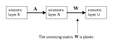
| [ < ] | [ > ] | [ << ] | [ Up ] | [ >> ] | [Top] | [Contents] | [Index] | [ ? ] |
For each of S, X and U we define a layer of nodes. Each layer is given a type and a set of default node characteristics. For A and W we define a projection between a pair of layers. Each projection is given a type and a set of default connection characteristics.
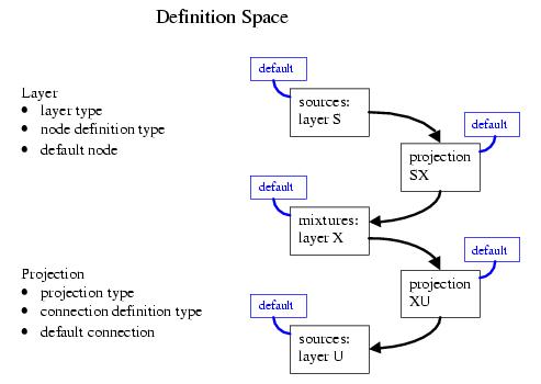
| [ < ] | [ > ] | [ << ] | [ Up ] | [ >> ] | [Top] | [Contents] | [Index] | [ ? ] |
Looking at the backend code for this we have:
create Plane_Spk S config S region=2:1 |
The first line creates an object of class Plane_Spk called S. Plane_Spk is a simple layer class, representing the layer as a two-dimensional plane of spiking nodes. The second line sets the size of the layer to be 2 nodes by 1 node.
S is the input layer in the model. The nodes will not have any synaptic inputs nor will they receive any injected currents. Instead we will define their activity by a probability distribution over their firing rates. We will later define this probability distribution and add a mechanism forcing the nodes in S to fire accordingly. We therefore do not have to define for layer S any further details regarding spike generation or synaptic integration mechanisms. This is not the case for layers X and U, which receive synaptic inputs. For X and U we define for the default node: an absolute refractory period, whether the membrane potential is reset to its base level after firing, and a threshold mechanism with a relative refractory period defined as Cthresh. The default node object for each layer is created automatically along with each layer object.
create Plane_Spk X create Plane_Spk U config X,U region=2:1 default/absref=0.001 default/memory=true default/threshold=Cthresh |
The Cthresh threshold mechanism in turn requires a kernel function and a limit to be defined. We first create an exponential function object to be used as the kernel function.
create Exp refractoryFunc tadapt=-0.02 config X,U default/thresh:func=refractoryFunc default/thresh:limit=0.15 |
create Planarproj_Psp SX from=S to=X create Planarproj_Psp XU from=X to=U |
For the default connection type we define a post-synaptic potential (PSP) function and an associated limit. We first create an instance of type Psp which models a piecewise linear PSP.
create Psp ica-psp rising=0.002 falling=0.058 config SX,XU default/psp=ica-psp default/limit=0.06 |
Finally we may wish to initialise the synaptic weights according to a probability distribution. We first define the distribution WDist. We use value expansion to associate the distribution with the weight for the default connection.
create Unif WDist lower=-0.25 upper=0.25 config SX,XU default/weight=@WDist@ |
This creates an object for each layer, projection and set of default parameters. At this stage we have defined only what is the model we want to build. We have not defined how we want to implement the model.
| [ < ] | [ > ] | [ << ] | [ Up ] | [ >> ] | [Top] | [Contents] | [Index] | [ ? ] |
In the frontend, much of this complexity could be hidden within library functions that define layers and projections.
nodeType=Spk
connType=Psp
layerSize=2
nConfig="default/absref=0.001 default/memory=true default/threshold=Cthresh default/thresh:func=refractoryFunc default/thresh:limit=0.15"
weights="Unif lower=-0.25 upper=0.25"
wConfig="default/weight=@WDist@"

fDefineLayer $nodeType S plane node region=${layerSize}:1
fDefineLayer $nodeType S plane node region=${layerSize}:1 $nConfig
fDefineLayer $nodeType S plane node region=${layerSize}:1 $nConfig

fCreateDistribution W $weights
fDefineProjection $connType SX planar S X $wConfig
fDefineProjection $connType XU planar X U $wConfig
|
| [ < ] | [ > ] | [ << ] | [ Up ] | [ >> ] | [Top] | [Contents] | [Index] | [ ? ] |
The next step is to take the design for the model and implement it. Assume that we wish to break the implementation up into two networks where each network has its own set of threads and each network computes one of the projections. This represents an allocation of computational resources to different parts of the model. The networks communicate using channel objects. A build object is used to define, effect and manage this allocation.
| [ < ] | [ > ] | [ << ] | [ Up ] | [ >> ] | [Top] | [Contents] | [Index] | [ ? ] |
The next step is to take the design for the model and implement it. First we create the two network objects. We choose networks of type Srnetev_P_S, which are networks of spike response neurons, implemented using an event-driven algorithm, communicating between networks using a packet protocol and running on a single thread. Next we create two build objects for networks of nodes of type Spk and connections of type Psp. The type of the build object is important as it defines the types of layers and projections that may be attached to it. A network object is associated with each build object.
create Srnetev_P_S XNet create Srnetev_P_S UNet create Build_SpkPspNet XBuild network=XNet create Build_SpkPspNet UBuild network=UNet |
Next we associate layers and projections with each build object.
config XBuild layerproj=S config XBuild layerproj=X config UBuild layerproj=U |
Next we resolve all of the projections against the available layers to check for inconsistencies, then we generate the implementation and finally we generate any required inter-network communication channels.
ex Gbuild resproj ex Gbuild gen ex global chanproj |
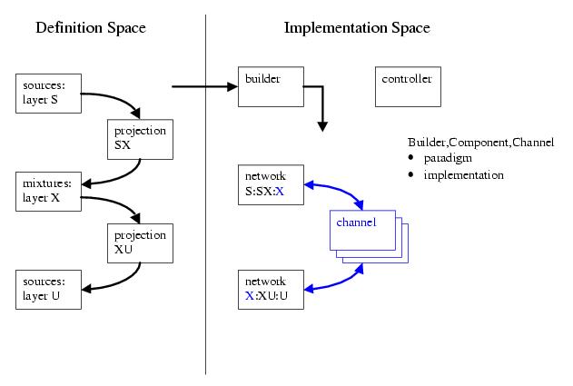
| [ < ] | [ > ] | [ << ] | [ Up ] | [ >> ] | [Top] | [Contents] | [Index] | [ ? ] |
We could choose to implement the whole model within a single network. In this case we would require only a single build object:
create Srnetev_P_S NNet create Build_SpkPspNet NBuild network=NNet config NBuild layerproj=S,X,U ex Gbuild resproj ex Gbuild gen ex global chanproj |
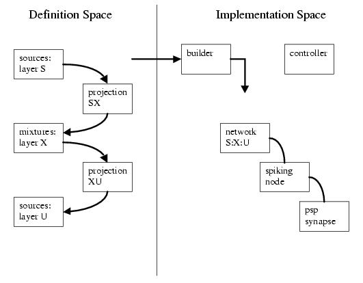
| [ < ] | [ > ] | [ << ] | [ Up ] | [ >> ] | [Top] | [Contents] | [Index] | [ ? ] |
After generating the implementation, the network will reference a set of newly created node objects, each of which will reference a set of newly created connection objects. Each of these node and connection objects can be referenced by name using relative addressing. For example, the connection to the second node in the U layer from the first node in the X layer is given by:
U/node/1/conn/X:0 |
Note that all indicies start from 0 not 1. This naming is valid for both the single and dual network implementations. Equivalent addressings for the single network implementation would be:
NNet/node/5/conn/0 NNet/node/U:1/conn/X:0 |
These addressing will change with the implementation. Equivalent addressings for the dual network implementation would be:
UNet/node/2/conn/0 UNet/node/U:1/conn/X:0 |
| [ < ] | [ > ] | [ << ] | [ Up ] | [ >> ] | [Top] | [Contents] | [Index] | [ ? ] |
The next step is to set up the inputs and outputs for the simulation. Each node in S must be attached to a distribution that defines the firing rate for the source. In addition, we need to measure the activities of each of the nodes in S, X and U.
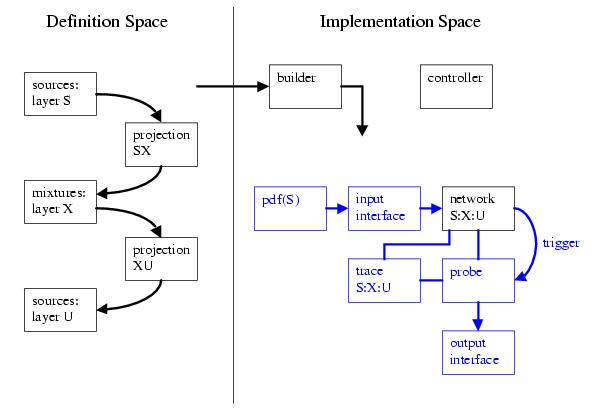
| [ < ] | [ > ] | [ << ] | [ Up ] | [ >> ] | [Top] | [Contents] | [Index] | [ ? ] |
The activity of any identifiable parameter can be recorded using a Probe object. Identifiable parameters are listed by name in the definition for each object class. Parameters are referenced using the same naming mechanisms as objects. A Probe object can also be used to measure the output of an object.
A probe object can be created explicitly and is given a name in the global address space. Some objects such as Network objects also have a probe command and an associated naming mechanism. A probe created by a probe command is given a tag or identifier so that it can be referenced from the creating object as well as by its global name. This is the preferred method for creating probes as it allows them to be meaningfully referenced from the network structure that they are attached to. A Probe object should only have attached parameters related to a single component object. This is because the probe mechanism uses a pointer mechanism and is not thread safe. Different components reflect different threads of execution.
ex NNet probe active=post tag=Probe time config NNet object/Probe/period=10000 |
Here a Probe object is created which can be referenced from NNet using the identifier "Probe". The last option "time" defines a parameter to be probed, in this case the current time for NNet. A probe may be attached to a trigger which can be used to activate the probe automatically. In this case the probe is activated on the "post" trigger for NNet, which means at the end of each time step. This is probably too frequently, so we can configure the probe to only take measurements once in every 10,000 activations. With a time step of 100 microseconds this corresponds to a sampling rate of 1 Hz.
Now that we have a probe set up, we need to attach a trace mechanism to each node that will calculate some continuous measure of spike activity. When the probe is activated it will have to activate each of these trace objects in turn and record the output of each. We can use the trace command for a node to create the traces, in this case we use traces of type Strace, which defines a simple firing rate measure over a given period. The "exists" option specifies the period and requests to use an existing trace if one exists. The "alink" option is passed as a configuration string to each newly created trace object, and specifies that it is to link itself to a new parameter slot in the probe object. The "owner" naming token is used to reference the owner of the trace, ie the node object, while the "network" naming token is used to reference the network associated with the node.
ex NNet node/S,X,U/trace exists=0.1 type=Strace alink=owner/network/object/Probe/param:new |
| [ < ] | [ > ] | [ << ] | [ Up ] | [ >> ] | [Top] | [Contents] | [Index] | [ ? ] |
We now have the probe set up, but we must still attach an output interface to the probe which defines what to do with the output. All input and output is done through interface objects. Derived interfaces exist for input and output to streams, input and output to files, and input from other objects. Interfaces can be bundled together and applied as a group, to reflect the definition of a specific input/output regime.
create Soface Record-NNet-Probe-Face strm=:Record-NNet-Probe.asc |
To manage a group of interfaces we create a Cfgset object and add a mapping between the probe and the interface.
create Cfgset RecordCfg config RecordCfg map=NNet-Probe,interface,Record-NNet-Probe-Face |
At a later stage we will attach the interfaces using:
ex RecordCfg apply |
| [ < ] | [ > ] | [ << ] | [ Up ] | [ >> ] | [Top] | [Contents] | [Index] | [ ? ] |
We create a distribution to define the firing rates of the nodes in S. We choose a laplacian distribution centred at 50 Hz with a variance of 5 Hz.
create Laplace SBaseDist first=50 second=5 lower=0.1 upper=1000 |
There are a number of ways to attach this distribution to the nodes in S. If S was defined as a layer of pins instead of a layer of nodes we could wrap an interface around the distribution and attach it to each of the pins. The method we use here is to create a base firing rate mechanism which defines a minimal level of firing. As the nodes in S have no synaptic inputs, then the base firing rate mechanism will define the firing activity for the nodes.
The approach is to utilise the parameters "next" and "last" together with the "fire" trigger, for a spiking node. The "next" parameter can be used to define the time in the future by which the node must next fire. If the synaptic input is not sufficient to cause the node to fire then the node will be forced to fire regardless of its membrane potential. By default, this parameter is initialised as being an infinite time into the future. By periodically setting this parameter we can ensure a base level of activity, even in the absence of synaptic input. The "last" parameter defines the time at which the node last fired, whilst the trigger "fire" is activated whenever the node fires.
With these attributes we can use a very simple Modop object to implement a base firing rate mechanism. For each node we create and attach a Modop object which updates "next" whenever the node fires. This Modop object obtains the value for "next" by adding a sample from the distribution function to "last". The sample from the distribution is interpreted as a firing rate and is used to generate an inter-spike interval that can be added to "last" to calculate "next".
ex S_build/network/*/make type=Netobj_Spkev tag=SBase mapto=network ex S_build/network/*/object/SBase/bind obj=S objtype=Modop objlink=fire objbind=next:next,last:last op=SBaseDist spikemode=rate |
The Modop objects are managed by collecting them under a Netobj_Spkev object. This allows the base rate objects to be collectively activated and de-activated. A single Netobj_Spkev object is created for each required network using the make command, as this allows each to be referenced from the relevant network.
This is an example of how a simple object can be used to implement a fairly complex mechanism by taking advantage of the identifiable parameters and triggers within the system. The advantage over coding the mechanism directly into the class and using a switch is the efficiency and reusability of the code. The advantage over coding the mechanism directly into a derived class is the avoidance of a combinatorial explosion in the number of classes and the flexibility provided to the user at run-time. The disadvantage is the complexity required in the software to handle the deletion of the associated pointer references along with the deletion of an object.
| [ < ] | [ > ] | [ << ] | [ Up ] | [ >> ] | [Top] | [Contents] | [Index] | [ ? ] |
The next step is to attach an object of type Ngica_Spkev to the network which implements the ICA learning algorithm for spiking neurons. Though this object will have a global name, it would be preferable if we could reference it through the network it is attached to. In multiple network models, each network that requires a learning algorithm must have its own instance of the learning class. A single instance of a learning algorithm class may not be shared by multiple networks due to thread safety. We therefore create the Ngica_Spkev object using the "make" object command for a network. We include some basic configuration.
ex NNet make type=Ngica_Spkev tag=Ica mapto=network config NNet adaptfactor=0.0 lrate=0.01 mode=online prior=IcaPriorDist period=1000 lrate=0.0001 |
The ICA algorithm will be applied to the U layer which is implemented in a single network, NNet. We could avoid requiring explicit knowledge of how layer U is implemented by using the following naming:
ex U build/network/*/make type=Ngica_Spkev tag=Ica mapto=network config U build/network/* adaptfactor=0.0 lrate=0.01 mode=online prior=IcaPriorDist period=1000 lrate=0.0001 |
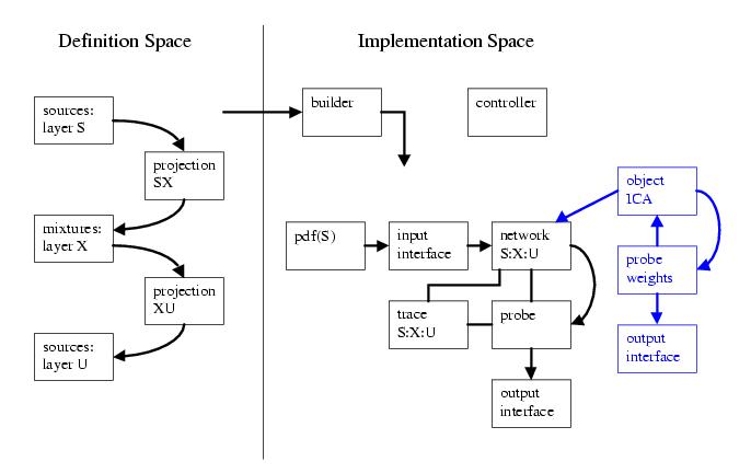
The next step is to bind the X and U nodes to the ICA object. A requirement of the algorithm is that a spiking node is bound to the algorithm through a trace object, as the algorithm is applied not to the underlying spike trains, but to continuous measures derived from the spike trains. It is necessary therefore to first create a trace mechanism, using the identifier "Ica", for each of the U nodes that can be used in the binding.
ex U node/*/trace id=Ica type=Strace period=0.05 ex U build/network/*/object/Ica/bind trace=Ica to=U from=X |
The final step is to set up a probe that will record what is happening during the learning. The probe is created and referenced from the Ngica_Spkev object, and is activated on the "post_iter" trigger or after every application of the algorithm. The parameters to probe are given as the time of the network, the modifiable connection weights and the continuous measures derived from the spike trains for the nodes in the layer U.
ex U build/network/*/object/Ica/probe active=post_iter network/time parameters uvalues. config U build/network/*/object/Ica/object/Probe/period=10 |
We set up an interface for the probe so that it will be activated and deactivated along with the other interfaces.
create Soface Record-NNet-Ica-Probe-Face strm=:Record-NNet-Ica-Probe.asc config RecordCfg map=NNet-Ica-Probe,interface,Record-NNet-Ica-Probe-Face |
| [ < ] | [ > ] | [ << ] | [ Up ] | [ >> ] | [Top] | [Contents] | [Index] | [ ? ] |
Basic initialisation includes defining the iteration time-steps for the simulation, the synchronisation time-step and the degree of parallelisation to use.
config Component timestep=0.0001 config default-controller synchstep=0.0001 concurrency=3 |
The next step is to reset the simulation.
ex Component,Controller,System reset ex Interface reset ex Probe reset |
The final steps are to activate the probes and learning algorithms. All learning algorithms for Spkev type spiking networks are derived from the Netbind_Spkev class.
config Netbind_Spkev active=true config Probe active=true |
The simulation can now be run forward for the required number of time-steps.
ex default-controller run loops=250000 |
| [ < ] | [ > ] | [ << ] | [ Up ] | [ >> ] | [Top] | [Contents] | [Index] | [ ? ] |
Consider building a network of spiking neurons to model the granular layer of the cerebellum. For learning, we will include a rule based on the level of extra-cellular calcium in the glomeruli. For details on the physiology of the model refer to foo.
| [ < ] | [ > ] | [ << ] | [ Up ] | [ >> ] | [Top] | [Contents] | [Index] | [ ? ] |
We define a layer of nodes for each of the mossy fibres, the granule cells and the golgi cells. Because the glomeruli are the junction for the mossy fibre terminals, the golgi cell axons and the granule cell dendrites, we define the glomeruli as a layer of nodes. This allows the use of existing projection objects in defining the relationship between mossy fibres and the glomeruli, and the golgi cell axons and the glomeruli. A single projection is also defined from the glomeruli to the granular cells. We assume at this stage, that the model is homogeneous, in that the same node and connection model is being used for all of the cells. The mossy fibres are the inputs to the system and therefore the mossy fibre nodes are used only as pins.
Whilst this model provides the necessary flexibility in determining the connectivity, there are a number of issues with respect to the standard model of nodes and connections. Firstly, the model must be homogenous implying that each node must include a membrane potential and a threshold mechanism, even though the glomeruli are not neurons. The glomeruli are distinct from the golgi and granule cells in that the inputs they receive from the mossy fibres and golgi cells must be passed through to the granule cells. Secondly, each connection between a glomerulus and a granule cell must be able to accomodate and distinguish between two types of inputs, mossy fibre inputs and golgi cell inputs.
To handle this, we introduce a new type of parameterised event-driven spiking node _Pspkevent, together with a multi-channel connection that that models multiple post-synaptic potential functions.
The projections between from the mossy fibres and the golgi cells to the glomeruli are defined using delta function PSP functions. The weights are chosen to satisfy two conditions. Firstly, that mossy fibre and golgi cell spikes are guaranteed to be passed through the threshold mechanism in the glomeruli to the granule cells with a delay of not more than a single time step. The structure of the membrane potential for each glomerulus is that of the combined spike trains for all of its mossy fibre and golgi cell inputs. Secondly, that the threshold mechanism in the glomeruli can decode the membrane potential back in to the separate spike trains, and passing the mossy fibre spikes to one channel in the projection to the granular layer, and the passing the golgi cell spikes to a second channel. Each spike produced by the threshold mechanism in a glomerulus is parameterised with the channel id. This channel id parameter is passed along with the spike to the connection, to allow the spike to be interpreted as either an inhibitory golgi cell spike or an excitatory mossy fibre spike.
The mossy fibre to glomeruli weights are given a weight of 1, the golgi cell to glomeruli weights are given a weight of 16, and the glomeruli are given a decoding threshold (Decthresh) mechanism with a base of 16. Two channels are defined for the glomeruli to granular cell projection, and a single channel is defined for all remaining projections.
config Gl/node/*/iconn/Mf:* weight=1.0 ex Gl/node/*/network make tag=MfGl-psp type=Delta width=0.0001 config Gl/node/*/iconn/Mf:* psp=onode/network/object/MfGl-psp config Gl/node/*/iconn/Go:* weight=16.0 ex Gl/node/*/network make tag=GoGl-psp type=Delta width=0.0001 config Gl/node/*/iconn/Go:* psp=onode/network/object/GoGl-psp ex Gl/node/* threshold type=Decthresh base=16.0 config Gr/node/*/iconn/Gl:* pathways=2 |
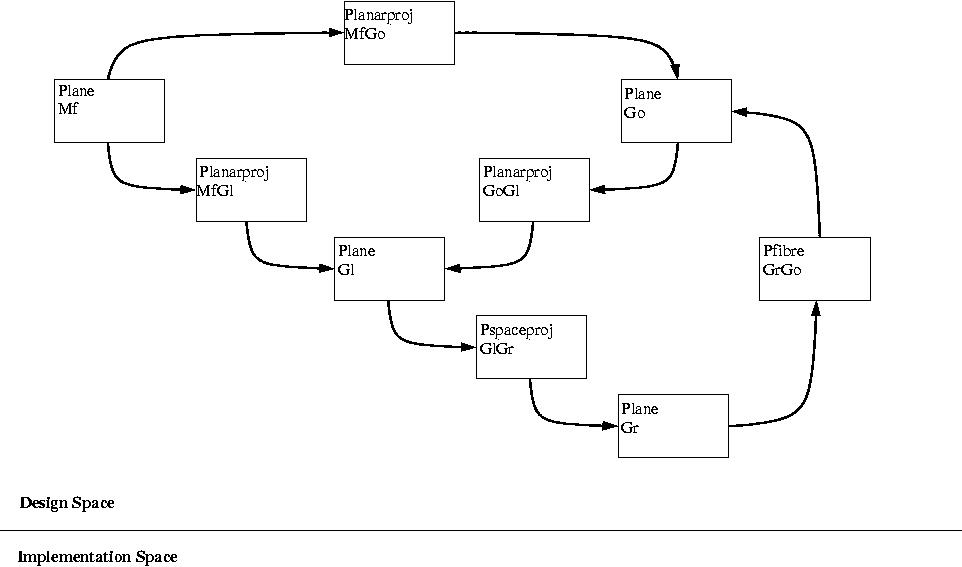
We define a conventional threshold mechanism with a relative refractory period for the golgi and granule cells. The default threshold mechanism and node configuration is sufficient for the mossy fibre nodes as at a later stage we will define their firing behaviour by a probability distribution.
| [ < ] | [ > ] | [ << ] | [ Up ] | [ >> ] | [Top] | [Contents] | [Index] | [ ? ] |
The next step is to bind objects to the network to implement the required synaptic plasticity.
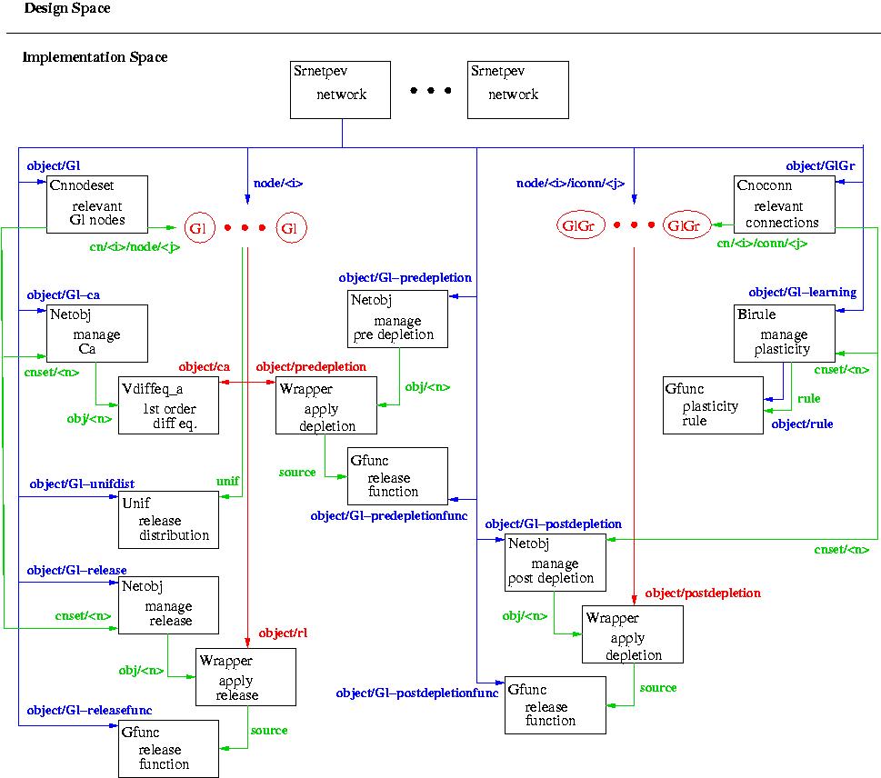
The figure shows how the different objects are structured in to trees where the root of each tree is a component. The blue and red lines show ownership while the green lines show references. The red lines indicate objects that are generated automatically by the bind commands.
The first step is to model the concentration of the Ca in each glomeruli, which can vary between 0 and 1. The replenishment of the Ca is given by a first order differential equation. We use a Netobj object to manage a collection of Vdiffeq_a objects, with a single Vdiffeq_a object being used to represent the Ca for a single glomerulus. The Netobj object must be listed with the network so that the Vdiffeq_a objects will be called periodically to calculate the replenishment. The time constant for the replenishment is dependent on the virtual time-scale defined by the calling period for the Netobj object.
ex Gl/build/network/* make type=derive:Netobj tag=Gl-ca cnset=owner/object/Gl list=true ${glCaConfig}
ex Gl/build/network/*/object/Gl-ca bind objtag=ca ${glCaBind}
|
The second step is to make the neurotransmitter release at the glomeruli probablilistic for both mossy fibre and golgi cell spikes. We use a Netobj object to attach a release probability mechanism to each glomeruli.
ex Gl/build/network/* make type=derive:Netobj tag=Gl-release cnset=owner/object/Gl list=false
ex Gl/build/network/* make tag=Gl-releasefunc ${glReleaseFunc}
ex Gl/build/network/*/object/Gl-release bind objtype=Wrapper objtag=rl objlink=release source=owner/network/object/Gl-releasefunc
|
The release probability mechanism is a function of the ca concentration.
ex Gl/build/network/*/object/Gl-release/obj/*/parameters passive reference=param:new source=owner/owner/object/ca/variable |
The release probability mechanism requires a random distribution
ex Gl/build/network/* make type=Unif tag=Gl-unifdist lower=0.0 upper=1.0 config Gl/build/network/*/object/Gl/cn/*/node/* unif=network/object/Gl-unifdist |
The third step is to model the change in extra-cellular Ca due to spikes in the mossy fibre terminals, the golgi cell axons and the granule cells. We use Netobj objects to manage collections of objects to manipulate the Ca concentrations. The Netobj objects must not be listed with the network as the Vdiffeq_a objects will be triggered when either the glomeruli, for the mossy fibre and golgi cell spikes, or the granule cells fire. For the mossy fibre and golgi cell spikes, this triggering will occur after the probability of neurotransmitter release has been calculated. For the mossy fibre and golgi cell spikes, the changes must be calculated when the spikes reach the glomeruli, not when they the spikes are generated at the respective somas, because of possible synaptic time delays. This requires a Wrapper object parameterised on the type of spike at the glomerulus to calculate the source-specific change in Ca concentration.
ex Gl/build/network/* make type=derive:Netobj tag=Ca-predepletion cnset=owner/object/Gl list=false
ex Gl/build/network/* make tag=Ca-predepletionfunc ${glPredepletionFunc}
ex Gl/build/network/*/object/Ca-predepletion bind objtype=Wrapper objtag=predepletion objlink=fire source=owner/network/object/Ca-predepletionfunc
|
The depletion mechanism is a function of the spike type parameter and the ca concentration.
ex Gl/build/network/*/object/Ca-predepletion/obj/*/parameters passive reference=param:new source=owner/owner/parameter ex Gl/build/network/*/object/Ca-predepletion/obj/*/parameters passive reference=param:new source=owner/owner/object/ca/variable |
The depletion mechanism must modify the ca concentration
ex Gl/build/network/*/object/Ca-predepletion/obj/* passive reference=output source=owner/object/ca/variable |
For the granule cell spikes, a change in Ca at the glomerulus is calculated for each glomerulus connected to the granule cell. This change is dependent on the weight of the synapse. We use a Cniconn object to define the set of granule cell synapses. For each synapse, a Wrapper object parameterised on the synaptic weight modifies the Ca concentration.
ex Gl/build/network/* make type=derive:Cnoconn tag=GlGr
ex Gl/build/network/*/object/GlGr bind post=Gr:* pre=Gl:* addpre=false addpost=false
ex Gl/build/network/* make type=derive:Netobj tag=Ca-postdepletion cnset=owner/object/GlGr list=false
ex Gl/build/network/* make tag=Ca-postdepletionfunc ${glPostdepletionFunc}
ex Gl/build/network/*/object/Ca-postdepletion bind objtype=Wrapper objtag=postdepletion objlink=onode/fire source=owner/inode/network/object/Ca-postdepletionfunc
|
The depletion mechanism is a function of the synaptic weight and the ca concentration.
ex Gl/build/network/*/object/Ca-postdepletion/obj/*/parameters passive reference=param:new source=owner/owner/pathway/0/weight ex Gl/build/network/*/object/Ca-postdepletion/obj/*/parameters passive reference=param:new source=owner/owner/inode/object/ca/variable |
The depletion mechanism must modify the ca concentration
ex Gl/build/network/*/object/Ca-postdepletion/obj/* passive reference=output source=owner/inode/object/ca/variable |
The fourth step is to model the plasticity of the granule cell synapses as a function of the Ca concentrations at the glomeruli. For this we use a Birule learning object that periodically calculates the weight changes for the synapses. We define the rule using a generic function object.
ex Gr/build/network/* make type=derive:Birule tag=Gr-learning cnset=owner/object/GlGr list=true ${glCalearnConfig}
ex Gr/build/network/*/object/Gr-learning make tag=rule ${glCalearnRule}
ex Gr/build/network/*/object/Gr-learning bind varone=pathway/0/weight vartwo=inode/object/ca/variable rule=object/rule parameter=pathway/0/weight ${glCalearnBind}
|
ex Activate-learning reg-config particles=Gr/build/network/*/object/Gr-learning active=true ex Deactivate-learning reg-config particles=Gr/build/network/*/object/Gr-learning active=false |
| [ < ] | [ > ] | [ << ] | [ Up ] | [ >> ] | [Top] | [Contents] | [Index] | [ ? ] |
typically this results from problems with the LD_LIBRARY_PATH environment variable.
Ensure that it references the correct libraries for the specific compiler that was used during the building.
Try running the backend directly. There could be problems with the message passing between the backend and the binary executables used by the frontend. Refer to the libthrio documentation for debugging the message passing streams. One option is to try communicating to the backend using a different frontend (see 7.1.4 Binding to a Backend.
In particular, the utility mqclean can be used to remove all message passsing streams belonging to the user, though note that this will cause all simulations to terminate.
A useful sequence of clean-up commands is mqclean, slay tennsS, slay tenns, slay xexit, mqclean.
| [ < ] | [ > ] | [ << ] | [ Up ] | [ >> ] | [Top] | [Contents] | [Index] | [ ? ] |
| Jump to: | B C E F G H I L M N O P Q S T U V |
|---|
| Jump to: | B C E F G H I L M N O P Q S T U V |
|---|
| [Top] | [Contents] | [Index] | [ ? ] |
| [Top] | [Contents] | [Index] | [ ? ] |
1. Notices
2. Introduction
3. Installation
4. Overview
5. Heterogenous Systems
6. About Models
7. Using TENNS
8. Tutorial
9. Troubleshooting
Concept Index
| [Top] | [Contents] | [Index] | [ ? ] |
| Button | Name | Go to | From 1.2.3 go to |
|---|---|---|---|
| [ < ] | Back | previous section in reading order | 1.2.2 |
| [ > ] | Forward | next section in reading order | 1.2.4 |
| [ << ] | FastBack | previous or up-and-previous section | 1.1 |
| [ Up ] | Up | up section | 1.2 |
| [ >> ] | FastForward | next or up-and-next section | 1.3 |
| [Top] | Top | cover (top) of document | |
| [Contents] | Contents | table of contents | |
| [Index] | Index | concept index | |
| [ ? ] | About | this page |